

Live notebook
You can run this notebook in a live session ![]() or view it on Github.
or view it on Github.
Extrapolate projection centers from a mean#
In this tutorial, we will extrapolate a plane of projection centers (PCs) from a mean PC. The PCs are determined from patterns spread out across the sample region of interest (ROI). This is an alternative to fitting a plane to PCs, as is demonstrated in the tutorial Fit a plane to selected projection centers. As a validation of the extrapolated PCs, we will compare them to the PCs obtained from fitting a plane to the PCs.
We’ll start by importing the necessary libraries
[1]:
%matplotlib inline

import matplotlib.pyplot as plt
import numpy as np

from diffsims.crystallography import ReciprocalLatticeVector
import hyperspy.api as hs
import kikuchipy as kp
from orix.crystal_map import PhaseList

plt.rcParams.update(
    {
        "figure.facecolor": "w",
        "figure.dpi": 75,
        "figure.figsize": (8, 8),
        "font.size": 15,
    }
)
Load and inspect data#
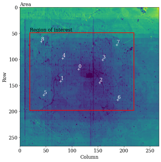
We will use nine calibration patterns from recrystallized nickel. The patterns are acquired with a NORDIF UF-1100 EBSD detector with the full (480, 480) px\(^2\) resolution. These patterns should always be acquired from spread out sample positions across the ROI in order to calibrate the PCs prior to indexing the full dataset.
Read the calibration patterns
[2]:
s_cal = kp.data.ni_gain_calibration(1, allow_download=True)
s_cal
[2]:
<EBSD, title: Calibration patterns, dimensions: (9|480, 480)>
Get information read from the NORDIF settings file
[3]:
omd = s_cal.original_metadata.as_dictionary()
Plot coordinates of calibration patterns on the secondary electron area overview image (part of the dataset), highlighting the ROI
[4]:
kp.draw.plot_pattern_positions_in_map(
    rc=omd["calibration_patterns"]["indices_scaled"],
    roi_shape=omd["roi"]["shape_scaled"],
    roi_origin=omd["roi"]["origin_scaled"],
    area_shape=omd["area"]["shape_scaled"],
    area_image=omd["area_image"],
    color="w",
)
Improve signal-to-noise ratio by removing the static and dynamic background
[5]:
s_cal.remove_static_background("divide")
s_cal.remove_dynamic_background("divide")
[########################################] | 100% Completed | 105.55 ms
[########################################] | 100% Completed | 105.78 ms
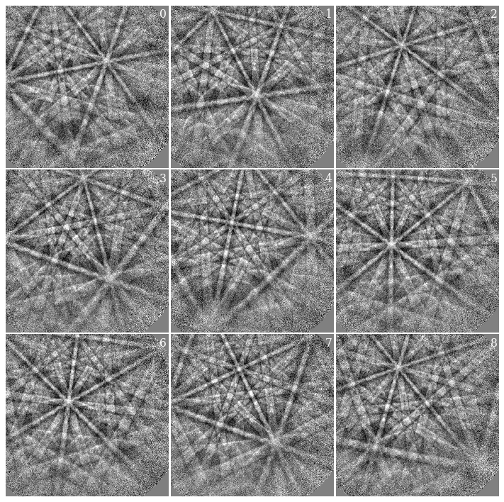
Let’s plot the nine background-corrected calibration patterns.
Before we do that, though, we find a suitable signal mask. The mask should exclude parts of the pattern without Kikuchi diffraction. Previous EBSD experiments on the microscope showed that the maximum intensity on the detector is a little to the left of the detector center. We therefore use a circular mask to exclude intensities in the upper and lower right corners of the detector
[6]:
r_pattern = kp.filters.distance_to_origin(
    s_cal.axes_manager.signal_shape[::-1], origin=(230, 220)
)
signal_mask = r_pattern > 310  # Exclude pixels set to True
For visual display only, we normalize intensities to a mean of 0 and a standard deviation of 1. We also exclude extreme intensities outside the range [-3, 3].
[7]:
s_cal2 = s_cal.normalize_intensity(dtype_out="float32", inplace=False)
[########################################] | 100% Completed | 105.59 ms
[8]:
fig = plt.figure(figsize=(12, 12))
_ = hs.plot.plot_images(
    s_cal2 * ~signal_mask,
    per_row=3,
    axes_decor=None,
    colorbar=False,
    label=None,
    fig=fig,
    vmin=-3,
    vmax=3,
)
for i, ax in enumerate(fig.axes):
    ax.axis("off")
    ax.text(475, 10, str(i), va="top", ha="right", c="w")
fig.subplots_adjust(wspace=0.01, hspace=0.01)
We know that all patterns are of nickel. To get a description of nickel, we could create a Phase manually. However, we will later on use a dynamically simulated EBSD master pattern of nickel (created with EMsoft), which is loaded with a Phase. We will use this in the remaining analysis.
[9]:
mp = kp.data.ebsd_master_pattern(
    "ni", allow_download=True, projection="lambert", energy=20
)
mp
[9]:
<EBSDMasterPattern, title: ni_mc_mp_20kv, dimensions: (|1001, 1001)>
Extract the phase, and change the lattice parameter unit from nm to Ångström
[10]:
phase = mp.phase

lat = phase.structure.lattice
lat.setLatPar(lat.a * 10, lat.b * 10, lat.c * 10)
<name: ni. space group: Fm-3m. point group: m-3m. proper point group: 432. color: tab:blue>
lattice=Lattice(a=3.5236, b=3.5236, c=3.5236, alpha=90, beta=90, gamma=90)
28   0.000000 0.000000 0.000000 1.0000
Estimate PCs with Hough indexing#
We will estimate PCs for the nine calibration patterns using PyEBSDIndex. See the Hough indexing tutorial for more details.
Note
PyEBSDIndex is an optional dependency of kikuchipy, and can be installed with both pip and conda (from conda-forge). To install PyEBSDIndex, see their installation instructions.
We need an EBSDIndexer to use PyEBSDIndex. We can obtain an indexer by passing a PhaseList to EBSDDetector.get_indexer(). Therefore, we need an initial EBSD detector
EBSDDetector(shape=(480, 480), pc=(0.5, 0.5, 0.5), sample_tilt=70.0, tilt=0.0, azimuthal=0.0, binning=1.0, px_size=1.0 um)
70.0
[13]:
Id  Name  Space group  Point group  Proper point group     Color
 0    ni        Fm-3m         m-3m                 432  tab:blue
[14]:
ni
0.05
We estimate the PC of each pattern with Hough indexing, and plot both the mean and standard deviation of the resulting PCs. Note that Bruker’s PC convention is used in kikuchipy. (We will “overwrite” the existing detector variable.)
[15]:
PC found: [********* ] 9/9  global best:0.167  PC opt:[0.4433 0.2216 0.4876]
[0.42216687 0.21743387 0.49994755]
[0.00800011 0.00469789 0.00506804]
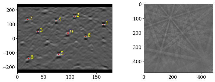
Plot the PCs
[16]:
det_cal.plot_pc("scatter", annotate=True)
Unfortunately, we do not recognize the spatial distribution from the overview image above. The expected inverse relation between (PCz, PCy) is not present either. We can try to improve indexing by refining the PCs using dynamical simulations. These simulations are created with EMsoft.
First, we need an initial guess of the orientations, which we get using Hough indexing via EBSD.hough_indexing(). We will use the mean PC for all patterns
[17]:
indexer.PC = det_cal.pc_average
[18]:
xmap_hi = s_cal.hough_indexing(pl, indexer=indexer, verbose=2)
Hough indexing with PyEBSDIndex information:
  PyOpenCL: True
  Projection center (Bruker): (0.4222, 0.2174, 0.4999)
  Indexing 9 pattern(s) in 1 chunk(s)
Radon Time: 0.010771750006824732
Convolution Time: 0.01894658402306959
Peak ID Time: 0.0209323339513503
Band Label Time: 0.01811941701453179
Total Band Find Time: 0.06899608299136162
Band Vote Time:  0.004288083000574261
  Indexing speed: 107.72150 patterns/s
Phase  Orientations  Name  Space group  Point group  Proper point group     Color
    0    9 (100.0%)    ni        Fm-3m         m-3m                 432  tab:blue
Properties: fit, cm, pq, nmatch
Scan unit: um
0.2611126
Refine PCs with pattern matching#
Refine the PCs (and orientations) using the Nelder-Mead implementation from NLopt
[20]:
xmap_ref, det_ref = s_cal.refine_orientation_projection_center(
    xmap=xmap_hi,
    detector=det_cal,
    master_pattern=mp,
    signal_mask=signal_mask,
    energy=20,
    method="LN_NELDERMEAD",
    trust_region=[5, 5, 5, 0.05, 0.05, 0.05],
    rtol=1e-6,
    # A pattern per iteration to use all CPUs
    chunk_kwargs=dict(chunk_shape=1),
)
Refinement information:
  Method: LN_NELDERMEAD (local) from NLopt
  Trust region (+/-): [5.   5.   5.   0.05 0.05 0.05]
  Relative tolerance: 1e-06
Refining 9 orientation(s) and projection center(s):
[########################################] | 100% Completed | 10.45 ss
Refinement speed: 0.86086 patterns/s
Inspect some refinement statistics
[21]:
print("Score mean:                ", xmap_ref.scores.mean())
print("Mean number of evaluations:", xmap_ref.num_evals.mean())
print("PC mean:     ", det_ref.pc.mean(0))
print("PC std:      ", det_ref.pc.std(0))
print("PC max. diff:", abs(det_cal.pc - det_ref.pc).max(0))

angles = xmap_hi.orientations.angle_with(xmap_ref.orientations, degrees=True)
print("Ori. max. diff [deg]:", angles.max())
Score mean:                 0.522740877336926
Mean number of evaluations: 373.22222222222223
PC mean:      [0.42067614 0.21330182 0.50037893]
PC std:       [0.00257266 0.00181229 0.00066377]
PC max. diff: [0.01919128 0.01695695 0.01228939]
Ori. max. diff [deg]: 1.3070797993248584
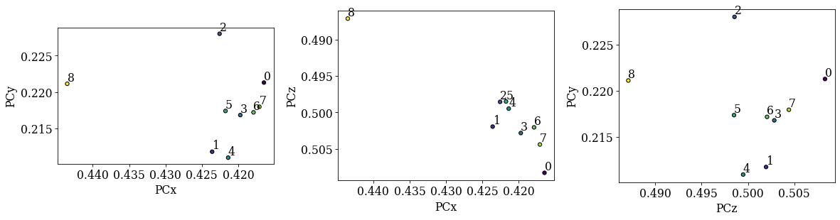
[22]:
det_ref.plot_pc("scatter", annotate=True)
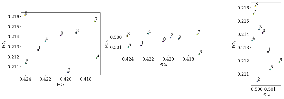
The diagonals 5-1-0-3-7 and 8-4-0-2-6 seen in the overview image above should be replicated in the (PCx, PCy) scatter plot. We see that 5-1-0-3-7 and 8-0-6 align as expected, but the PC values from the 2nd and 4th patterns do not lie in the expected range. Fitting a plane to all these values might not work to our satisfaction, so we will exclude the 2nd and 4th PC values when fitting a plane to the seven remaining PC values. The plane will have PC values for all points in the ROI in the overview image above.
Get PC plane by fitting#
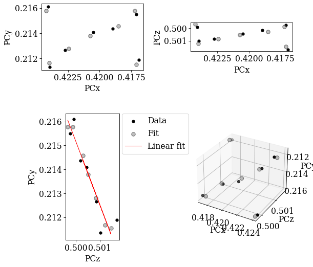
The fitting is done by finding a transformation function which takes 2D sample coordinates and gives PC values for those coordinates. Both an affine and a projective transformation function is supported, following [Winkelmann et al., 2020]. By passing 2D indices of all ROI map points and of the points where the nine calibration patterns were obtained, EBSDDetector.fit_pc() returns a new detector with PC values for all map points. We will use the maximum difference between the above refined PC values and the corresponding fitted PC values as a measure of how good the fitted PC values are.
[24]:
pc_indices = omd["calibration_patterns"]["indices_scaled"]
pc_indices -= omd["roi"]["origin_scaled"]
pc_indices = pc_indices.T

map_indices = np.indices(omd["roi"]["shape_scaled"])
print("Full map shape (n rows, n columns):", omd["roi"]["shape_scaled"])
Full map shape (n rows, n columns): (149, 200)
Fit PC values using the affine transformation function
[25]:
[0.4204937  0.21363595 0.50058975]
68.94100264528139
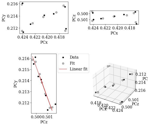
Fit PC values using the projective transformation function
[26]:
[0.42048979 0.21363086 0.50059015]
70.09817931001172
Compare PC differences of all but the PC values from the 2nd and 4th patterns
[27]:
pc_indices2 = pc_indices.T[~is_outlier].T

# Refined PC values as a reference (ground truth)
pc_ref = det_ref.pc[~is_outlier]

# Difference in PC values from the affine transformation function
pc_diff_aff = det_fit_aff.pc[tuple(pc_indices2)] - pc_ref
pc_diff_aff_max = abs(pc_diff_aff).max(axis=0)
print(pc_diff_aff_max)

# Difference in PC values from the projective transformation function
pc_diff_proj = det_fit_proj.pc[tuple(pc_indices2)] - pc_ref
pc_diff_proj_max = abs(pc_diff_proj).max(axis=0)
print(pc_diff_proj_max)

# Which fitted PCs are more different from refined PCs, the projective (True)
# or the affine (False)?
print(pc_diff_proj_max > pc_diff_aff_max)
[0.00044063 0.00047204 0.00027505]
[0.00045682 0.00042079 0.00028141]
[ True False  True]
Get PC plane by extrapolation#
Instead of fitting a plane to several PCs, we can extrapolate an average PC using EBSDDetector.extrapolate_pc(). To do this we need to know the detector pixel size and map step sizes, both given in the same unit.
[28]:
[0.41957349 0.21404736 0.50043583]
70.0
Difference in PC values between the refined PCs and the corresponding extrapolated PCs
[29]:
[0.00152036 0.00078621 0.00042069]
[ True  True  True]
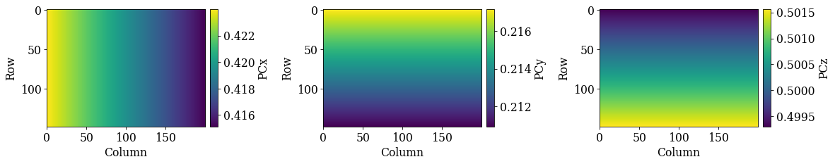
The extrapolated PCs deviate more from the refined PCs than the PCs obtained from fitting, although the difference is small.
[30]:
det_ext.plot_pc()
Validate extrapolated PCs#
As a final check of the difference in PCs, we can plot the geometrical simulations on top of the patterns using the refined orientation but the three different PCs.
[31]:
g = ReciprocalLatticeVector.from_min_dspacing(phase.deepcopy())

g.sanitise_phase()  # "Fill atoms in the unit cell"

g.calculate_structure_factor()

F = abs(g.structure_factor)
g = g[F > 0.5 * F.max()]

g.print_table()
 h k l      d     |F|_hkl   |F|^2   |F|^2_rel   Mult
 1 1 1    2.034    11.8     140.0     100.0      8
 2 0 0    1.762    10.4     108.2      77.3      6
 2 2 0    1.246     7.4     55.0       39.3      12
 3 1 1    1.062     6.2     38.6       27.6      24
[32]:
Using PCs from the affine transformation function
[33]:
det_aff_cal = det_fit_aff.deepcopy()
det_aff_cal.pc = det_aff_cal.pc[tuple(pc_indices)]
[34]:
xmap_aff = s_cal.refine_orientation(
    xmap=xmap_hi,
    detector=det_aff_cal,
    master_pattern=mp,
    energy=20,
    signal_mask=signal_mask,
    method="LN_NELDERMEAD",
    trust_region=[5, 5, 5],
    rtol=1e-6,
    chunk_kwargs={"chunk_shape": 1},
)
Refinement information:
  Method: LN_NELDERMEAD (local) from NLopt
  Trust region (+/-): [5 5 5]
  Relative tolerance: 1e-06
Refining 9 orientation(s):
[########################################] | 100% Completed | 2.21 sms
Refinement speed: 4.06301 patterns/s
[35]:
sim_aff = simulator.on_detector(det_aff_cal, xmap_aff.rotations)
Finding bands that are in some pattern:
[########################################] | 100% Completed | 105.54 ms
Finding zone axes that are in some pattern:
[########################################] | 100% Completed | 106.04 ms
Calculating detector coordinates for bands and zone axes:
[########################################] | 100% Completed | 106.96 ms
Using PCs from the projective transformation function
[36]:
det_proj_cal = det_fit_proj.deepcopy()
det_proj_cal.pc = det_proj_cal.pc[tuple(pc_indices)]
[37]:
xmap_proj = s_cal.refine_orientation(
    xmap=xmap_hi,
    detector=det_proj_cal,
    master_pattern=mp,
    energy=20,
    signal_mask=signal_mask,
    method="LN_NELDERMEAD",
    trust_region=[5, 5, 5],
    rtol=1e-6,
    chunk_kwargs={"chunk_shape": 1},
)
Refinement information:
  Method: LN_NELDERMEAD (local) from NLopt
  Trust region (+/-): [5 5 5]
  Relative tolerance: 1e-06
Refining 9 orientation(s):
[########################################] | 100% Completed | 1.90 sms
Refinement speed: 4.72157 patterns/s
[38]:
sim_proj = simulator.on_detector(det_proj_cal, xmap_proj.rotations)
Finding bands that are in some pattern:
[########################################] | 100% Completed | 105.78 ms
Finding zone axes that are in some pattern:
[########################################] | 100% Completed | 106.72 ms
Calculating detector coordinates for bands and zone axes:
[########################################] | 100% Completed | 106.94 ms
Using the extrapolated PCs
[39]:
det_ext_cal = det_ext.deepcopy()
det_ext_cal.pc = det_ext_cal.pc[tuple(pc_indices)]
[40]:
xmap_ext = s_cal.refine_orientation(
    xmap=xmap_hi,
    detector=det_ext_cal,
    master_pattern=mp,
    energy=20,
    signal_mask=signal_mask,
    method="LN_NELDERMEAD",
    trust_region=[5, 5, 5],
    rtol=1e-6,
    chunk_kwargs={"chunk_shape": 1},
)
Refinement information:
  Method: LN_NELDERMEAD (local) from NLopt
  Trust region (+/-): [5 5 5]
  Relative tolerance: 1e-06
Refining 9 orientation(s):
[########################################] | 100% Completed | 2.22 sms
Refinement speed: 4.05478 patterns/s
[41]:
sim_ext = simulator.on_detector(det_ext_cal, xmap_ext.rotations)
Finding bands that are in some pattern:
[########################################] | 100% Completed | 105.67 ms
Finding zone axes that are in some pattern:
[########################################] | 100% Completed | 106.08 ms
Calculating detector coordinates for bands and zone axes:
[########################################] | 100% Completed | 106.94 ms
Compare normalized cross-correlation scores and number of evaluations (iterations)
[42]:
print("Scores\n------")
print(f"Affine:       {xmap_aff.scores.mean():.7f}")
print(f"Projective:   {xmap_proj.scores.mean():.7f}")
print(f"Extrapolated: {xmap_ext.scores.mean():.7f}\n")

print("Number of evaluations\n---------------------")
print(f"Affine:       {xmap_aff.num_evals.mean():.1f}")
print(f"Projective:   {xmap_proj.num_evals.mean():.1f}")
print(f"Extrapolated: {xmap_ext.num_evals.mean():.1f}")
Scores
------
Affine:       0.5225239
Projective:   0.5225153
Extrapolated: 0.5221928

Number of evaluations
---------------------
Affine:       114.1
Projective:   97.1
Extrapolated: 114.6
Plot Kikuchi bands on top of patterns for the solutions using the affine transformed PCs (red), projective transformed PCs (blue), and extrapolated PCs (white)
[43]:
fig, axes = plt.subplots(ncols=3, nrows=3, figsize=(12, 12))
for i, ax in enumerate(axes.ravel()):
    ax.imshow(
        s_cal2.inav[i].data * ~signal_mask, cmap="gray", vmin=-3, vmax=3
    )
    ax.axis("off")

    # Affine
    lines = sim_aff.as_collections(
        i, lines_kwargs={"linewidth": 4, "alpha": 0.4}
    )[0]
    ax.add_collection(lines)

    # Projective
    lines = sim_proj.as_collections(
        i, lines_kwargs={"color": "b", "linewidth": 3, "alpha": 0.4}
    )[0]
    ax.add_collection(lines)

    # Extrapolated
    lines = sim_ext.as_collections(
        i, lines_kwargs={"color": "w", "linewidth": 1, "alpha": 0.4}
    )[0]
    ax.add_collection(lines)

    ax.text(5, 10, i, c="w", va="top", ha="left", fontsize=20)
fig.subplots_adjust(wspace=0.01, hspace=0.01)
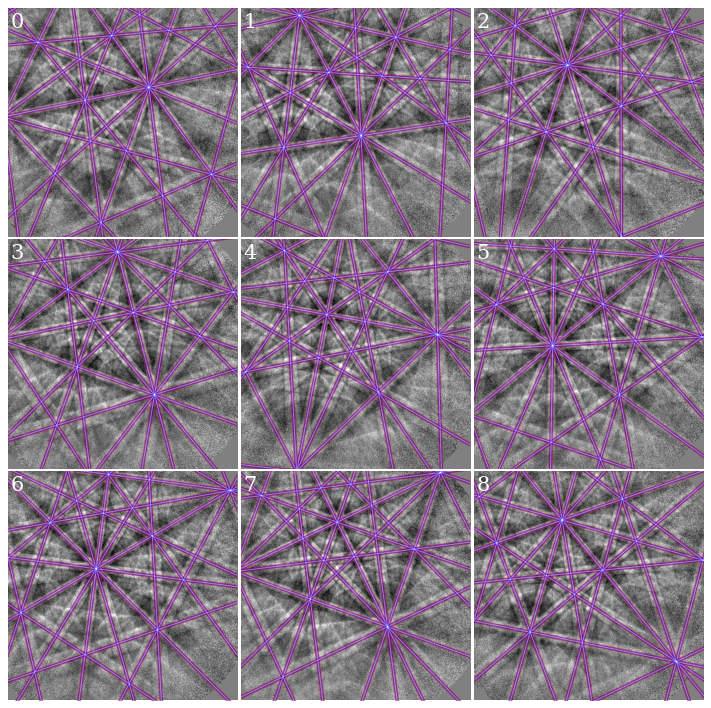
As expected from the intermediate results above (similar average PC and NCC score), all PCs produce visually identical geometrical simulations. However, the orientations may be slightly different
[44]:
xmap_proj.orientations.angle_with(xmap_ext.orientations, degrees=True).mean()
[44]:
0.10997283165066242
The estimated orientations using PCs from plane fitting are on average misoriented by about 1\(^{\circ}\) from the estimated orientations using extrapolated PCs. The misorientation is most likely a result of the difference in applied sample tilts
[45]:
abs(det_proj_cal.sample_tilt - det_ext_cal.sample_tilt)
[45]:
0.09817931001171587
Since these are experimental data, it’s difficult to say which sample tilt is more correct, although the nominal sample tilt from the microscope was 70\(^{\circ}\).