Plot distribution of projection centers

This example shows how to plot a distribution of projection/pattern centers (PCs) with the EBSDDetector. See the detector class documentation for further details on the definition of the PC and gnomonic coordinates.

Imports.

import matplotlib.pyplot as plt

import kikuchipy as kp

Create a detector with smoothly varying PC values, extrapolated from a single PC (assumed to be in the upper left corner of a map)

det0 = kp.detectors.EBSDDetector(
    shape=(480, 640), pc=(0.4, 0.3, 0.5), px_size=70, sample_tilt=70
)
print(det0)

det = det0.extrapolate_pc(
    pc_indices=[0, 0], navigation_shape=(5, 10), step_sizes=(20, 20)
)
print(det)

EBSDDetector
  shape (Ny, Nx):     (480, 640)
  pc (PCx, PCy, PCz): (0.4, 0.3, 0.5)
  sample_tilt:        70.0°
  tilt:               0.0°
  azimuthal:          0.0°
  twist:              0.0°
  binning:            1
  px_size:            70.0 um
EBSDDetector
  shape (Ny, Nx):     (480, 640)
  pc (PCx, PCy, PCz): (0.398, 0.299, 0.5)
  sample_tilt:        70.0°
  tilt:               0.0°
  azimuthal:          0.0°
  twist:              0.0°
  binning:            1
  px_size:            70.0 um

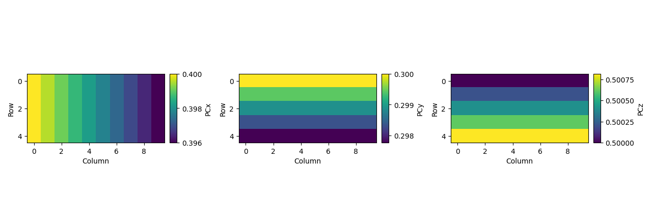
Plot PC values in maps.

det.plot_pc()

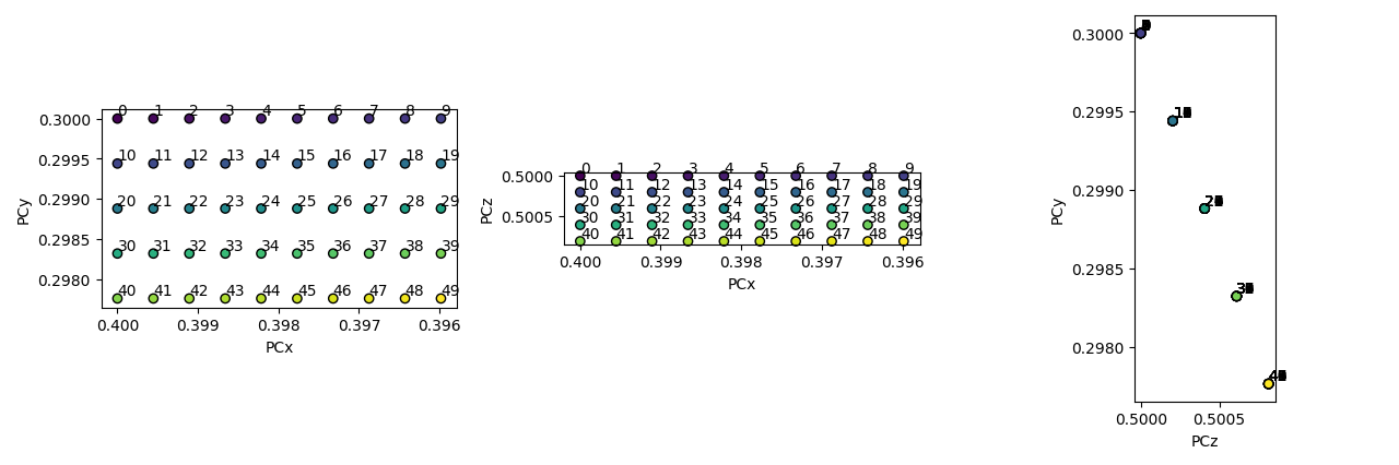
Plot in scatter plots in vertical orientation.

det.plot_pc("scatter", annotate=True)

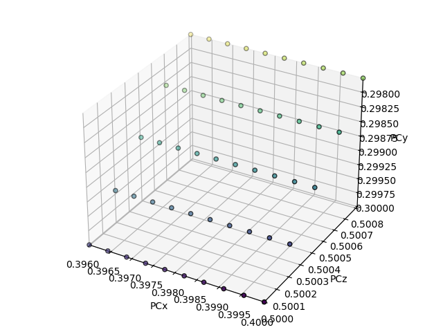
Plot in a 3D scatter plot, returning the figure for saving etc.

fig = det.plot_pc("3d", return_figure=True)

plt.show()

Estimated memory usage: 790 MB