Adaptive histogram equalization

This example shows how to perform AHE on a simulated pattern and a master pattern. Two identical simulated patterns, but one projected from the master pattern after AHE has been applied to it, are compared. We’ll use kikuchipy.signals.EBSDMasterPattern.adaptive_histogram_equalization() and the equivalent method for the EBSD class.

Adaptive histogram equalization (AHE) has been used to enhance pattern contrast and improve the efficacy of the normalized dot product (NDP) metric when comparing experimental and simulated patterns, e.g. in dictionary indexing [Marquardt et al., 2017]. Before performing AHE, it might be worth considering using the normalized cross-correlation (NCC) metric instead.

import hyperspy.api as hs
import kikuchipy as kp
import matplotlib.pyplot as plt
from mpl_toolkits.axes_grid1 import make_axes_locatable
from orix.quaternion import Rotation


hs.preferences.General.show_progressbar = False

# Master pattern in square Lambert projection, of integer data type
mp = kp.data.nickel_ebsd_master_pattern_small(projection="lambert")

mp2 = mp.adaptive_histogram_equalization(inplace=False)

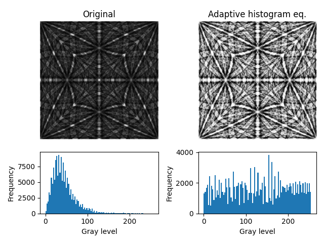
# Plot master pattern before and after correction and the intensity histograms
mps_data = [mp.data, mp2.data]
fig, axes = plt.subplots(2, 2, height_ratios=[3, 1.5])
for ax, pattern, title in zip(
    axes[0], mps_data, ["Original", "Adaptive histogram eq."]
):
    ax.imshow(pattern, cmap="gray")
    ax.set_title(title)
    ax.axis("off")
for ax, pattern in zip(axes[1], mps_data):
    ax.hist(pattern.ravel(), bins=100)
    ax.set(xlabel="Gray level", ylabel="Frequency")
fig.tight_layout()

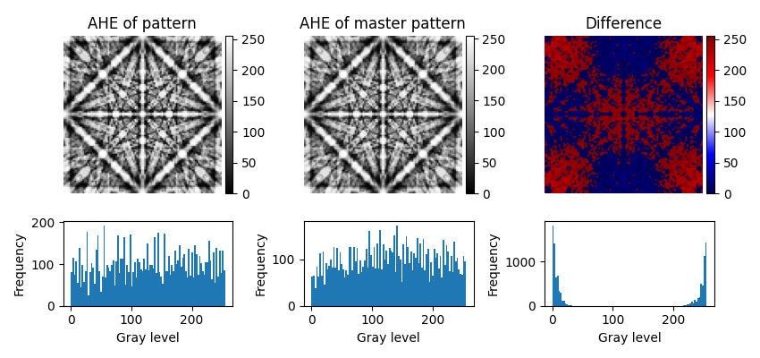
Let’s show that intensities are approximately the same in patterns where one is equalized while the other is projected from a master pattern which itself is equalized.

# Project experimental patterns from each master pattern
det = kp.detectors.EBSDDetector((100, 100), sample_tilt=0)
r = Rotation.identity()
s1 = mp.get_patterns(r, det, energy=20, dtype_out="uint8", compute=True)
s2 = mp2.get_patterns(r, det, energy=20, dtype_out="uint8", compute=True)

# Adaptive histogram equalization of the first pattern
s1.adaptive_histogram_equalization()

# Plot the patterns, their difference and their intensity histograms
patterns = [s1.data, s2.data, (s1 - s2).data]
fig, axes = plt.subplots(2, 3, figsize=(8.5, 4), height_ratios=[3, 1.5])
for ax, pattern, title, cmap in zip(
    axes[0],
    patterns,
    ["AHE of pattern", "AHE of master pattern", "Difference"],
    ["gray", "gray", "seismic"],
):
    im = ax.imshow(pattern.squeeze(), cmap=cmap)
    ax.set_title(title)
    ax.axis("off")
    divider = make_axes_locatable(ax)
    cax = divider.append_axes("right", size="5%", pad=0.05)
    plt.colorbar(im, cax=cax)
for ax, pattern in zip(axes[1], patterns):
    ax.hist(pattern.ravel(), bins=100)
    ax.set(xlabel="Gray level", ylabel="Frequency")
fig.tight_layout()

Estimated memory usage: 12 MB