Live notebook

You can run this notebook in a live session or view it on Github.

Pattern processing

The raw EBSD signal can be characterized as a superposition of a Kikuchi diffraction pattern and a smooth background intensity. For pattern indexing, the latter intensity is undesirable, while for virtual backscatter electron VBSE) imaging, this intensity can reveal topographical, compositional or diffraction contrast.

This tutorial details methods to enhance the Kikuchi diffraction pattern and manipulate detector intensities in patterns in an EBSD signal.

Most of the methods operating on EBSD objects use functions that operate on the individual patterns (numpy.ndarray). Some of these single pattern functions are available in the kikuchipy.pattern module.

Let’s import the necessary libraries and read the Nickel EBSD test data set

# Exchange inline for notebook or qt5 (from pyqt) for interactive plotting
%matplotlib inline

import matplotlib.pyplot as plt
import numpy as np

import hyperspy.api as hs
import kikuchipy as kp

# Use kp.load("data.h5") to load your own data
s = kp.data.nickel_ebsd_small()

Most methods operate inplace (indicated in their docstrings), meaning they overwrite the patterns in the EBSD signal. If we instead want to keep the original signal and operate on a new signal, we can either create a deepcopy() of the original signal…

s2 = s.deepcopy()
np.may_share_memory(s.data, s2.data)

False

… or pass inplace=False to return a new signal and keep the original signal unaffected (new in version 0.8).

Let’s make a convenience function to plot a pattern before and after processing with the intensity distributions below. We’ll also globally silence progressbars

def plot_pattern_processing(patterns, titles):
    """Plot two patterns side by side with intensity histograms below.

    Parameters
    ----------
    patterns : list of numpy.ndarray
    titles : list of str
    """
    fig, axes = plt.subplots(2, 2, height_ratios=[3, 1.5])
    for ax, pattern, title in zip(axes[0], patterns, titles):
        ax.imshow(pattern, cmap="gray")
        ax.set_title(title)
        ax.axis("off")
    for ax, pattern in zip(axes[1], patterns):
        ax.hist(pattern.ravel(), bins=100)
    fig.tight_layout()


hs.preferences.General.show_progressbar = False

Background correction

Remove the static background

Effects which are constant, like hot pixels or dirt on the detector, can be removed by subtracting or dividing by a static background wit remove_static_background()

s2 = s.remove_static_background(inplace=False)

plot_pattern_processing(
    [s.inav[0, 0].data, s2.inav[0, 0].data], ["Raw", "Static"]
)

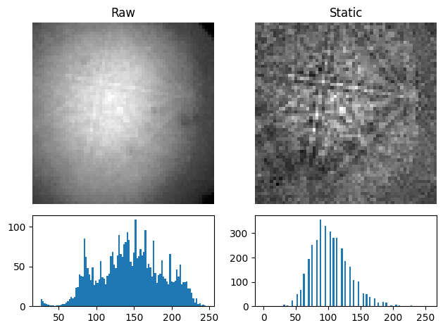
We didn’t have to pass a background pattern since it is stored with the currenct signal in the static_background attribute. We could instead pass the background pattern in the static_bg parameter.

The static background pattern intensity range can be scaled to each individual pattern’s range prior to removal with scale_bg=True.

Remove the dynamic background

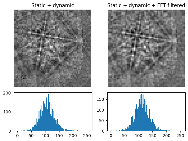
Uneven intensity in a static background subtracted pattern can be corrected by subtraction or division of a dynamic background pattern obtained by Gaussian blurring with remove_dynamic_background(). A Gaussian window with a standard deviation set by std is used to blur each pattern individually (dynamic) either in the spatial or frequency domain, set by filter_domain. Blurring in the frequency domain uses a low-pass Fast Fourier Transform (FFT) filter. Each pattern is then subtracted or divided by the individual dynamic background pattern depending on the operation

s3 = s2.remove_dynamic_background(
    operation="subtract",  # Default
    filter_domain="frequency",  # Default
    std=8,  # Default is 1/8 of the pattern width
    truncate=4,  # Default
    inplace=False,
)

plot_pattern_processing(
    [s2.inav[0, 0].data, s3.inav[0, 0].data], ["Static", "Static + dynamic"]
)

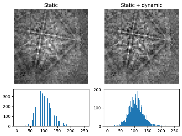
The width of the Gaussian window is truncated at the truncated number of standard deviations. Output patterns are rescaled to fill the input patterns’ data type range.

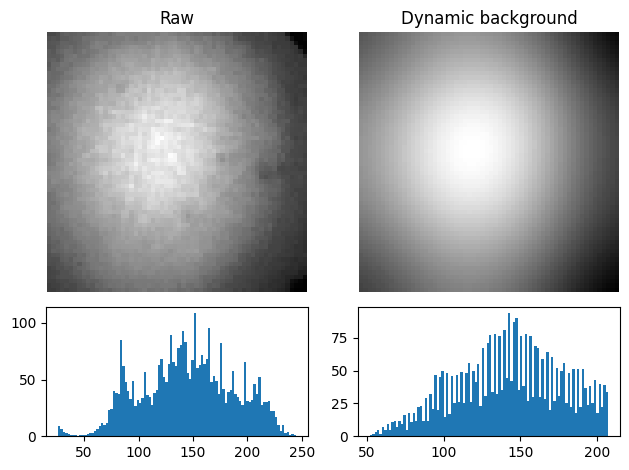
Get the dynamic background

The Gaussian blurred pattern removed during dynamic background correction can be obtained as an EBSD signal by calling get_dynamic_background()

bg = s.get_dynamic_background(filter_domain="frequency", std=8, truncate=4)

plot_pattern_processing(
    [s.inav[0, 0].data, bg.inav[0, 0].data], ["Raw", "Dynamic background"]
)

Average neighbour patterns

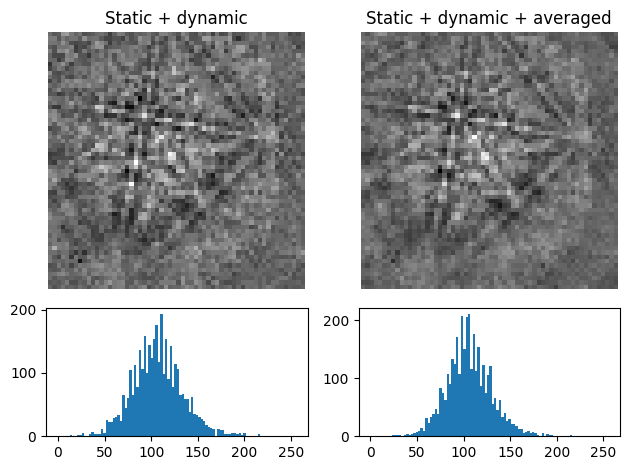
The signal-to-noise ratio in patterns in a scan can be improved by averaging patterns with their closest neighbours within a window/kernel/mask using average_neighbour_patterns()

s4 = s3.average_neighbour_patterns(window="gaussian", std=1, inplace=False)

plot_pattern_processing(
    [s3.inav[0, 0].data, s4.inav[0, 0].data],
    ["Static + dynamic", "Static + dynamic + averaged"],
)

The array of averaged patterns \(g(n_{\mathrm{x}}, n_{\mathrm{y}})\) is obtained by spatially correlating a window \(w(s, t)\) with the array of patterns \(f(n_{\mathrm{x}}, n_{\mathrm{y}})\), here 4D, which is padded with zeros at the edges. As coordinates \(n_{\mathrm{x}}\) and \(n_{\mathrm{y}}\) are varied, the window origin moves from pattern to pattern, computing the sum of products of the window coefficients with the neighbour pattern intensities, defined by the window shape, followed by normalizing by the sum of the window coefficients. For a symmetrical window of shape \(m \times n\), this becomes [Gonzalez and Woods, 2017]

\begin{equation} g(n_{\mathrm{x}}, n_{\mathrm{y}}) = \frac{\sum_{s=-a}^a\sum_{t=-b}^b{w(s, t) f(n_{\mathrm{x}} + s, n_{\mathrm{y}} + t)}} {\sum_{s=-a}^a\sum_{t=-b}^b{w(s, t)}}, \end{equation}

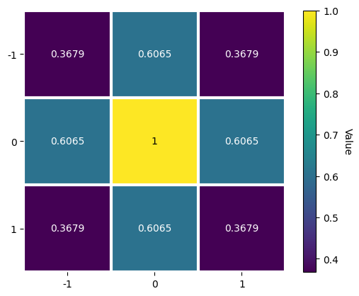
where \(a = (m - 1)/2\) and \(b = (n - 1)/2\). The window \(w\), a Window object, can be plotted

w = kp.filters.Window(window="gaussian", shape=(3, 3), std=1)
w.plot()

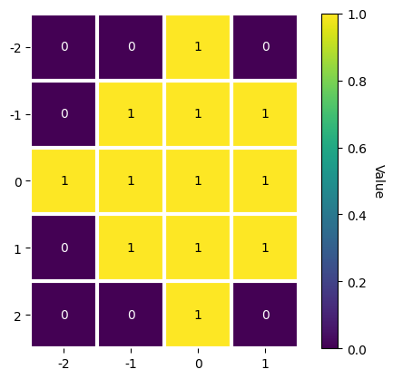
Any 1D or 2D window with desired coefficients can be used. This custom window can be passed to the window parameter in average_neighbour_patterns() or Window as a numpy.ndarray or a dask.array.Array. Additionally, any window in scipy.signal.windows.get_window() passed as a string via window with the necessary parameters as keyword arguments (like std=1 for window="gaussian") can be used. To demonstrate the creation and use of an asymmetrical circular window (and the use of make_circular(), although we could create a circular window directly by calling window="circular" upon window initialization)

w = kp.filters.Window(window="rectangular", shape=(5, 4))
w

Window (5, 4) rectangular
[[1. 1. 1. 1.]
 [1. 1. 1. 1.]
 [1. 1. 1. 1.]
 [1. 1. 1. 1.]
 [1. 1. 1. 1.]]

w.make_circular()
w.plot()

But this (5, 4) averaging window cannot be used with our (3, 3) navigation shape signal.

Note

Neighbour pattern averaging increases the virtual interaction volume of the electron beam with the sample, leading to a potential loss in spatial resolution. Averaging may in some cases, like on grain boundaries, mix two or more different diffraction patterns, which might be unwanted. See [Wright et al., 2015] for a discussion of this concern.

Adaptive histogram equalization

Enhancing the pattern contrast with adaptive histogram equalization has been found useful when comparing patterns for dictionary indexing [Marquardt et al., 2017]. With adaptive_histogram_equalization(), the intensities in the pattern histogram are spread to cover the available range, e.g. [0, 255] for patterns of uint8 data type

s6 = s3.adaptive_histogram_equalization(kernel_size=(15, 15), inplace=False)

plot_pattern_processing(
    [s3.inav[0, 0].data, s6.inav[0, 0].data],
    ["Static + dynamic", "Static + dynamic + adapt. hist. eq."],
)

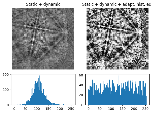
The kernel_size parameter determines the size of the contextual regions. See e.g. Fig. 5 in [Jackson et al., 2019], also available via EMsoft’s GitHub repository wiki, for the effect of varying kernel_size.

Filtering in the frequency domain

Filtering of patterns in the frequency domain can be done with fft_filter(). This method takes a spatial kernel defined in the spatial domain, or a transfer function defined in the frequency domain, in the transfer_function argument as a numpy.ndarray or a Window. Which domain the transfer function is defined in must be passed to the function_domain argument. Whether to shift zero-frequency components to the center of the FFT can also be controlled via shift, but note that this is only used when function_domain="frequency".

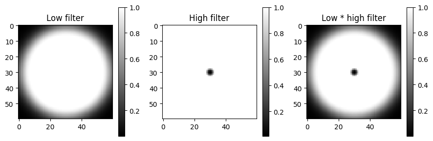
Popular uses of filtering of EBSD patterns in the frequency domain include removing large scale variations across the detector with a Gaussian high pass filter, or removing high frequency noise with a Gaussian low pass filter. These particular functions are readily available via Window

pattern_shape = s.axes_manager.signal_shape[::-1]
w_low = kp.filters.Window(
    window="lowpass", cutoff=23, cutoff_width=10, shape=pattern_shape
)
w_high = kp.filters.Window(
    window="highpass", cutoff=3, cutoff_width=2, shape=pattern_shape
)

fig, axes = plt.subplots(figsize=(9, 3), ncols=3)
for ax, data, title in zip(
    axes, [w_low, w_high, w_low * w_high], ["Low", "High", "Low * high"]
):
    im = ax.imshow(data, cmap="gray")
    ax.set_title(title + " filter")
    fig.colorbar(im, ax=ax)
fig.tight_layout()

Then, to multiply the FFT of each pattern with this transfer function, and subsequently computing the inverse FFT (IFFT), we use fft_filter(), and remember to shift the zero-frequency components to the centre of the FFT

s7 = s3.fft_filter(
    transfer_function=w_low * w_high,
    function_domain="frequency",
    shift=True,
    inplace=False,
)

plot_pattern_processing(
    [s3.inav[0, 0].data, s7.inav[0, 0].data],
    ["Static + dynamic", "Static + dynamic + FFT filtered"],
)

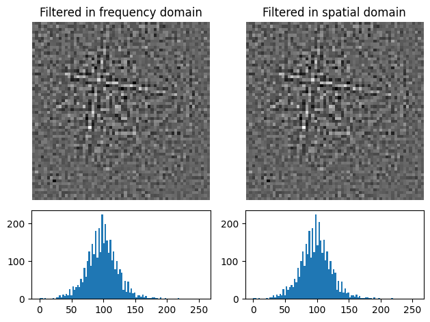
Note that filtering with a spatial kernel in the frequency domain, after creating the kernel’s transfer function via FFT, and computing the inverse FFT (IFFT), is, in this case, the same as spatially correlating the kernel with the pattern.

Let’s demonstrate this by attempting to sharpen a pattern with a Laplacian kernel in both the spatial and frequency domains and comparing the results (this is a purely illustrative example, and perhaps not that practically useful)

from scipy.ndimage import correlate


# fmt: off
w_laplacian = np.array([
    [-1, -1, -1],
    [-1,  8, -1],
    [-1, -1, -1]
])
# fmt: on
s8 = s3.fft_filter(
    transfer_function=w_laplacian, function_domain="spatial", inplace=False
)


p_filt = correlate(
    s3.inav[0, 0].data.astype(np.float32), weights=w_laplacian
)
p_filt_resc = kp.pattern.rescale_intensity(p_filt, dtype_out=np.uint8)

plot_pattern_processing(
    [s8.inav[0, 0].data, p_filt_resc],
    ["Filtered in frequency domain", "Filtered in spatial domain"],
)

np.sum(s8.inav[0, 0].data - p_filt_resc)  # Which is zero

1275

Note also that fft_filter() performs the filtering on the patterns with data type np.float32, and therefore have to rescale back to the pattern’s original data type if necessary.

Rescale intensity

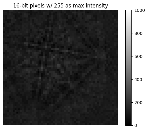
Vendors usually write patterns to file with 8 (uint8) or 16 (uint16) bit integer depth, holding [0, 2\(^8\)] or [0, 2\(^{16}\)] gray levels, respectively. To avoid losing intensity information when processing, we often change data types to e.g. 32 bit floating point (float32). However, only changing the data type with change_dtype() does not rescale pattern intensities, leading to patterns not using the full available data type range

s9 = s3.deepcopy()
print(s9.data.dtype, s9.data.max())

uint8 255

s9.change_dtype(np.uint16)
print(s9.data.dtype, s9.data.max())

uint16 255

plt.figure()
plt.imshow(s9.inav[0, 0].data, vmax=1000, cmap="gray")
plt.title("16-bit pixels w/ 255 as max intensity")
plt.axis("off")
_ = plt.colorbar()

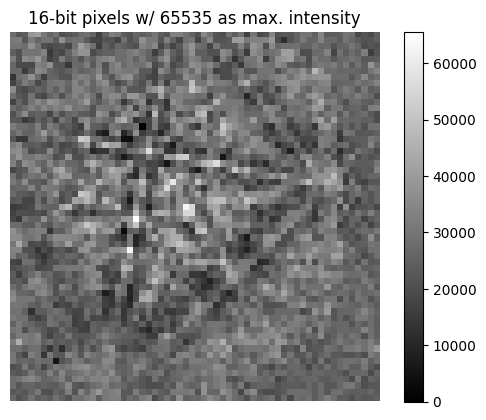
In these cases it is convenient to rescale intensities to a desired data type range, either keeping relative intensities between patterns in a scan or not. We can do this for all patterns in an EBSD signal with kikuchipy.signals.EBSD.rescale_intensity()

s9.rescale_intensity(relative=True)
print(s9.data.dtype, s9.data.max())

uint16 65535

plt.figure()
plt.imshow(s9.inav[0, 0].data, cmap="gray")
plt.title("16-bit pixels w/ 65535 as max. intensity")
plt.axis("off")
_ = plt.colorbar()

Or, we can do it for a single pattern (numpy.ndarray) with kikuchipy.pattern.rescale_intensity()

p = s3.inav[0, 0].data
print(p.min(), p.max())

0 255

p2 = kp.pattern.rescale_intensity(p, dtype_out=np.uint16)
print(p2.min(), p2.max())

0 65535

We can also stretch the pattern contrast by removing intensities outside a range passed to in_range or at certain percentiles by passing percentages to percentiles

print(s3.inav[0, 0].data.min(), s3.inav[0, 0].data.max())

0 255

s10 = s3.inav[0, 0].rescale_intensity(out_range=(10, 245), inplace=False)
print(s10.data.min(), s10.data.max())

10 245

s10.rescale_intensity(percentiles=(0.5, 99.5))
print(s10.data.min(), s3.data.max())

0 255

plot_pattern_processing(
    [s3.inav[0, 0].data, s10.data],
    ["Static + dynamic", "Static + dynamic + clip low/high"],
)

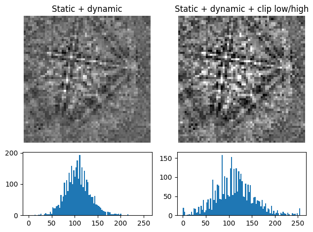
This can reduce the influence of outliers with exceptionally high or low intensities, like hot or dead pixels.

Normalize intensity

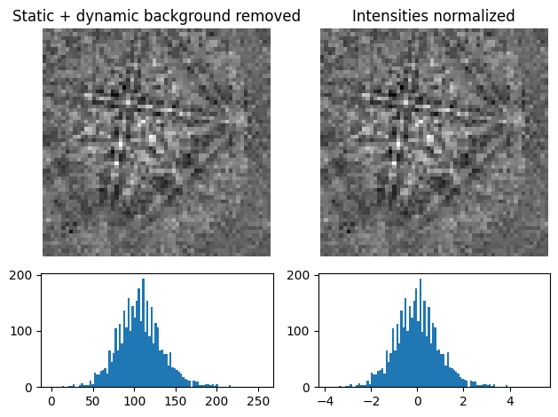
It can be useful to normalize pattern intensities to a mean value of \(\mu = 0.0\) and a standard deviation of e.g. \(\sigma = 1.0\) when e.g. comparing patterns or calculating the image quality. Patterns can be normalized with normalize_intensity()

np.mean(s3.inav[0, 0].data)

107.2775

s11 = s3.inav[0, 0].normalize_intensity(num_std=1, dtype_out=np.float32, inplace=False)
np.mean(s11.data)

0.0

plot_pattern_processing(
    [s3.inav[0, 0].data, s11.data],
    ["Static + dynamic background removed", "Intensities normalized"],
)