
Live notebook
You can run this notebook in a live session ![]() or view it on Github.
or view it on Github.
Geometrical EBSD simulations#
In this tutorial, we will inspect and visualize the results from EBSD indexing by plotting Kikuchi lines and zone axes onto an EBSD signal. We consider this a geometrical EBSD simulation, since it is only positions of Kikuchi lines and zone axes that are computed. These simulations are based on the work by Aimo Winkelmann in the supplementary material to [Britton et al., 2016].
These simulations can be helpful when checking whether indexing results are correct and for interpreting them.
Let’s import the necessary libraries
[1]:
# Exchange inline for notebook or qt5 (from pyqt) for interactive plotting
%matplotlib inline

import matplotlib.pyplot as plt
import numpy as np

from diffpy.structure import Atom, Lattice, Structure
from diffsims.crystallography import ReciprocalLatticeVector
import hyperspy.api as hs
import kikuchipy as kp
from orix.crystal_map import Phase

# Plotting parameters
plt.rcParams.update(
    {"figure.figsize": (10, 10), "font.size": 20, "lines.markersize": 10}
)
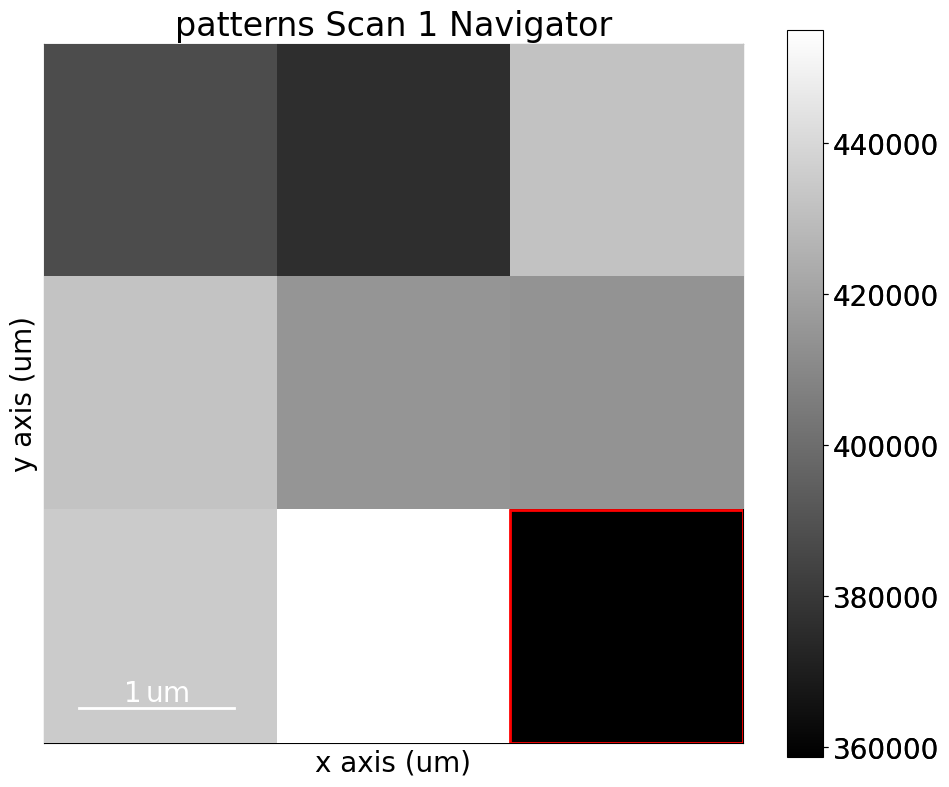
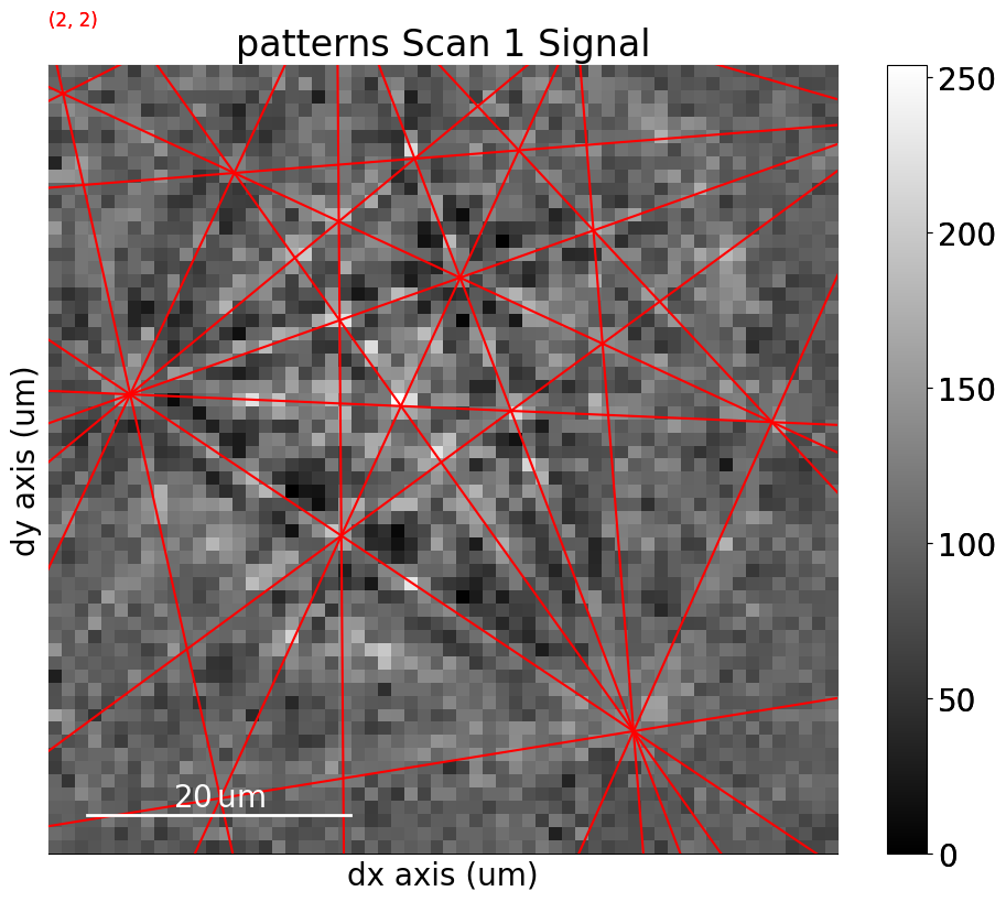
We’ll inspect the indexing results of a small nickel EBSD dataset of (3, 3) patterns
[2]:
# Use kp.load("data.h5") to load your own data
s = kp.data.nickel_ebsd_small()
s
[2]:
<EBSD, title: patterns Scan 1, dimensions: (3, 3|60, 60)>
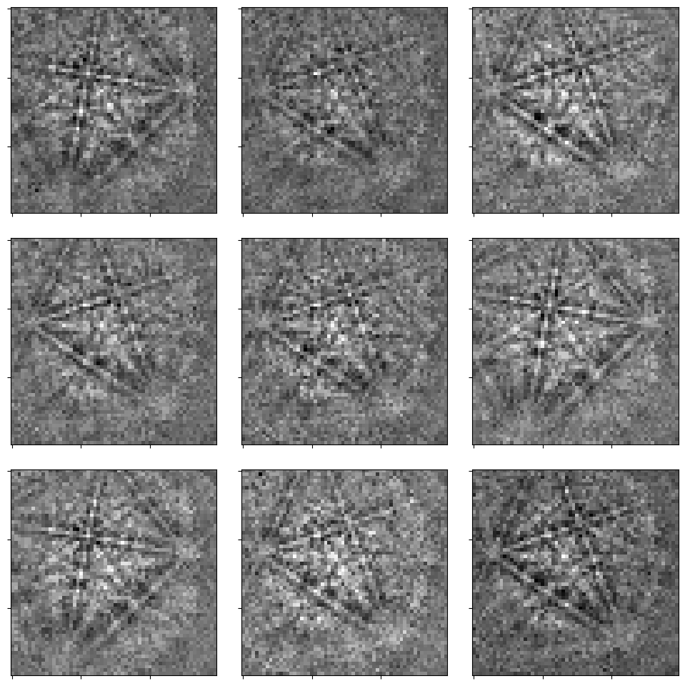
Let’s enhance the Kikuchi bands by removing the static and dynamic backgrounds
[3]:
s.remove_static_background()
s.remove_dynamic_background()
[4]:
_ = hs.plot.plot_images(
    s, axes_decor=None, label=None, colorbar=False, tight_layout=True
)
To project Kikuchi lines and zone axes onto our detector, we need
a description of the crystal phase
the set of Kikuchi bands to consider, e.g. the sets of planes {111}, {200}, {220}, and {311}
the crystal orientations with respect to the reference frame
the position of the detector with respect to the sample, in the form of a sample-detector model which includes the sample and detector tilt and the projection center (shortes distance from the source point on the sample to the detector), given here as (PC\(_x\), PC\(_y\), PC\(_z\))
Prepare phase and reflector list#
We’ll store the crystal phase information in an orix.crystal_map.Phase instance
[5]:
<name: . space group: Fm-3m. point group: m-3m. proper point group: 432. color: tab:blue>
lattice=Lattice(a=3.52, b=3.52, c=3.52, alpha=90, beta=90, gamma=90)
Ni   0.000000 0.000000 0.000000 1.0000
We’ll build up the reflector list using diffsims.crystallography.ReciprocalLatticeVector
[6]:
rlv = ReciprocalLatticeVector(
    phase=phase, hkl=[[1, 1, 1], [2, 0, 0], [2, 2, 0], [3, 1, 1]]
)
rlv
[6]:
ReciprocalLatticeVector (4,),  (m-3m)
[[1. 1. 1.]
 [2. 0. 0.]
 [2. 2. 0.]
 [3. 1. 1.]]
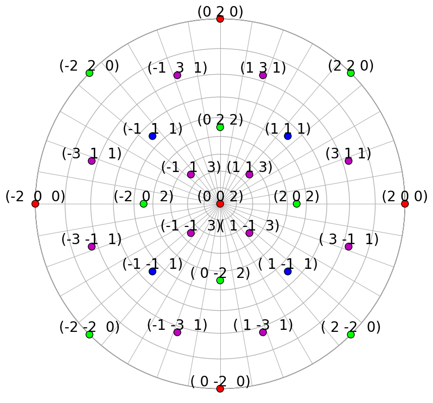
We’ll obtain the symmetrically equivalent vectors and plot each family of vectors in a distinct colour in the stereographic projection
[7]:
rlv = rlv.symmetrise().unique()
rlv.size
[7]:
50
[8]:
rlv.print_table()
 h k l      d     |F|_hkl   |F|^2   |F|^2_rel   Mult
 3 1 1    1.061     nan      nan       nan       24
 1 1 1    2.032     nan      nan       nan       8
 2 2 0    1.245     nan      nan       nan       12
 2 0 0    1.760     nan      nan       nan       6
[9]:
# Dictionary with {hkl} as key and indices into ReciprocalLatticeVector as values
hkl_sets = rlv.get_hkl_sets()
hkl_sets
[9]:
defaultdict(tuple,
            {(np.float64(2.0),
              np.float64(0.0),
              np.float64(0.0)): (array([ 8,  9, 10, 11, 12, 13]),),
             (np.float64(2.0),
              np.float64(2.0),
              np.float64(0.0)): (array([14, 15, 16, 17, 18, 19, 20, 21, 22, 23, 24, 25]),),
             (np.float64(1.0),
              np.float64(1.0),
              np.float64(1.0)): (array([0, 1, 2, 3, 4, 5, 6, 7]),),
             (np.float64(3.0),
              np.float64(1.0),
              np.float64(1.0)): (array([26, 27, 28, 29, 30, 31, 32, 33, 34, 35, 36, 37, 38, 39, 40, 41, 42,
                     43, 44, 45, 46, 47, 48, 49]),)})
[10]:
[11]:
[12]:
rlv.scatter(c=hkl_colors, grid=True, ec="k", vector_labels=hkl_labels)
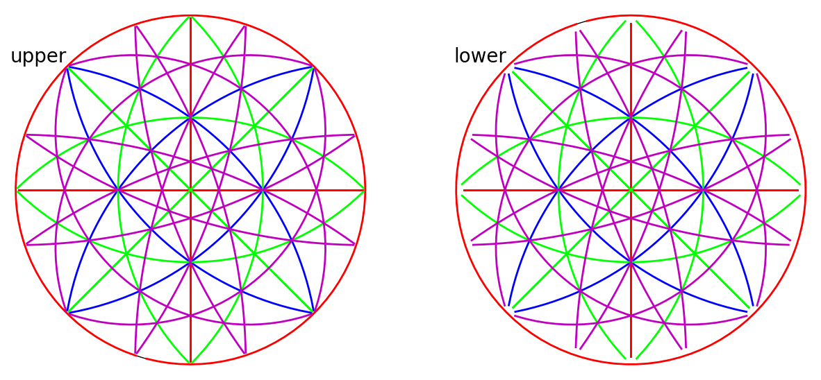
We can also plot the plane traces, i.e. the Kikuchi lines, in both hemispheres (they are identical for Ni)
[13]:
rlv.draw_circle(
    color=hkl_colors, hemisphere="both", figure_kwargs=dict(figsize=(15, 10))
)
Specify rotations and detector-sample geometry#
Rotations and the detector-sample geometry for the nine nickel EBSD patterns are stored in the kikuchipy h5ebsd file. These were found by Hough indexing using PyEBSDIndex followed by orientation and PC refinement using a nickel EBSD master pattern simulated with EMsoft. See the Hough indexing and Pattern matching tutorials for details on indexing and the reference frame tutorial for details on the definition of the detector-sample geometry.
[14]:
rot = s.xmap.rotations
rot = rot.reshape(*s.xmap.shape)
rot  # Quaternions
[14]:
Rotation (3, 3)
[[[ 0.8743  0.0555  0.475   0.083 ]
  [ 0.4745  0.2915  0.4221 -0.7153]
  [ 0.4761  0.2915  0.4232 -0.7136]]

 [[ 0.2686 -0.1295  0.6879 -0.6618]
  [ 0.4755  0.2923  0.4244 -0.713 ]
  [ 0.4773  0.2925  0.4251 -0.7113]]

 [[ 0.5608 -0.2951  0.3731  0.6776]
  [ 0.7103 -0.4248  0.294   0.4781]
  [ 0.2999  0.0357  0.7124  0.6335]]]
We describe the sample-detector model in an kikuchipy.detectors.EBSDDetector instance. The sample was tilted \(70^{\circ}\) about the microscope X direction towards the detector, and the detector normal was orthogonal to the optical axis (beam direction). Using this information, the projection center (PC) was found using PyEBSDIndex as described in the Hough indexing tutorial.
[15]:
s.detector
[15]:
EBSDDetector
  shape (Ny, Nx):     (60, 60)
  pc (PCx, PCy, PCz): (0.425, 0.213, 0.501)
  sample_tilt:        70.0°
  tilt:               0.0°
  azimuthal:          0.0°
  twist:              0.0°
  binning:            8
  px_size:            1.0 um
[16]:
s.detector.pc
[16]:
array([[[0.4214844 , 0.21500351, 0.50201974],
        [0.42414583, 0.21014019, 0.50104439],
        [0.42637843, 0.21145593, 0.5004183 ]],

       [[0.42088203, 0.2165417 , 0.50079336],
        [0.42725023, 0.21450546, 0.49996293],
        [0.43082231, 0.21369458, 0.50123367]],

       [[0.42194418, 0.21202927, 0.4997446 ],
        [0.43085722, 0.21436106, 0.50068903],
        [0.42248503, 0.21257126, 0.50045621]]])
Create simulations on detector#
Now we’re ready to create geometrical simulations. We create simulations using the kikuchipy.simulations.KikuchiPatternSimulator, which takes the reflectors as input
[17]:
[18]:
sim = simulator.on_detector(s.detector, rot)
Finding bands that are in some pattern:
[########################################] | 100% Completed | 101.29 ms
Finding zone axes that are in some pattern:
[########################################] | 100% Completed | 101.09 ms
Calculating detector coordinates for bands and zone axes:
[########################################] | 100% Completed | 101.20 ms
By passing the detector and crystal orientations to KikuchiPatternSimulator.on_detector(), we’ve obtained a kikuchipy.simulations.GeometricalKikuchiPatternSimulation, which stores the detector and gnomonic coordinates of the Kikuchi lines and zone axes for each crystal orientation
[19]:
[19]:
GeometricalKikuchiPatternSimulation (3, 3):
ReciprocalLatticeVector (49,),  (m-3m)
[[ 1.  1.  1.]
 [-1.  1.  1.]
 [-1. -1.  1.]
 [ 1. -1.  1.]
 [ 1. -1. -1.]
 [ 1.  1. -1.]
 [-1.  1. -1.]
 [-1. -1. -1.]
 [ 2.  0.  0.]
 [ 0.  2.  0.]
 [-2.  0.  0.]
 [ 0. -2.  0.]
 [ 0.  0.  2.]
 [ 0.  0. -2.]
 [ 2.  2.  0.]
 [-2.  2.  0.]
 [-2. -2.  0.]
 [ 2. -2.  0.]
 [ 0.  2.  2.]
 [-2.  0.  2.]
 [ 0. -2.  2.]
 [ 2.  0.  2.]
 [ 0.  2. -2.]
 [ 0. -2. -2.]
 [ 2.  0. -2.]
 [ 3.  1.  1.]
 [-1.  3.  1.]
 [-3. -1.  1.]
 [ 1. -3.  1.]
 [ 1.  3.  1.]
 [-3.  1.  1.]
 [-1. -3.  1.]
 [ 3. -1.  1.]
 [ 3. -1. -1.]
 [ 1.  3. -1.]
 [-3.  1. -1.]
 [-1. -3. -1.]
 [-1.  3. -1.]
 [-3. -1. -1.]
 [ 1. -3. -1.]
 [ 3.  1. -1.]
 [ 1. -1.  3.]
 [ 1.  1.  3.]
 [-1.  1.  3.]
 [-1. -1.  3.]
 [-1. -1. -3.]
 [ 1. -1. -3.]
 [ 1.  1. -3.]
 [-1.  1. -3.]]
We see that not all 50 of the reflectors in the reflector list are present in some pattern.
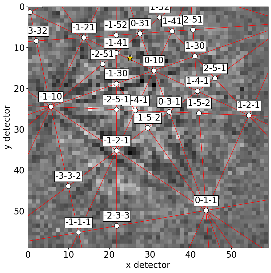
Plot simulations#
These geometrical simulations can be plotted one-by-one by themselves
[20]:
sim.plot()
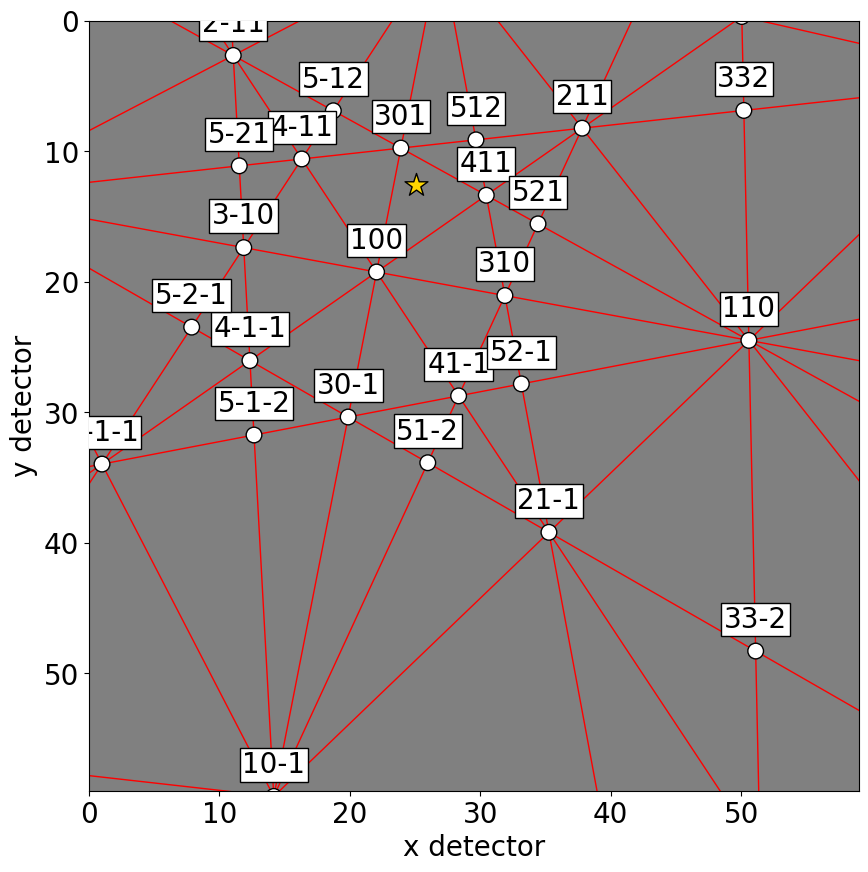
Or, they can be plotted on top of patterns in three ways: passing a pattern to GeometricalKikuchiPatternSimulation.plot()
[21]:
sim.plot(index=(1, 2), pattern=s.inav[2, 1].data)
Or, we can obtain collections of lines, zone axes and zone axes labels as Matplotlib objects via GeometricalKikuchiPatternSimulation.as_collections() and add them to an existing Matplotlib axis
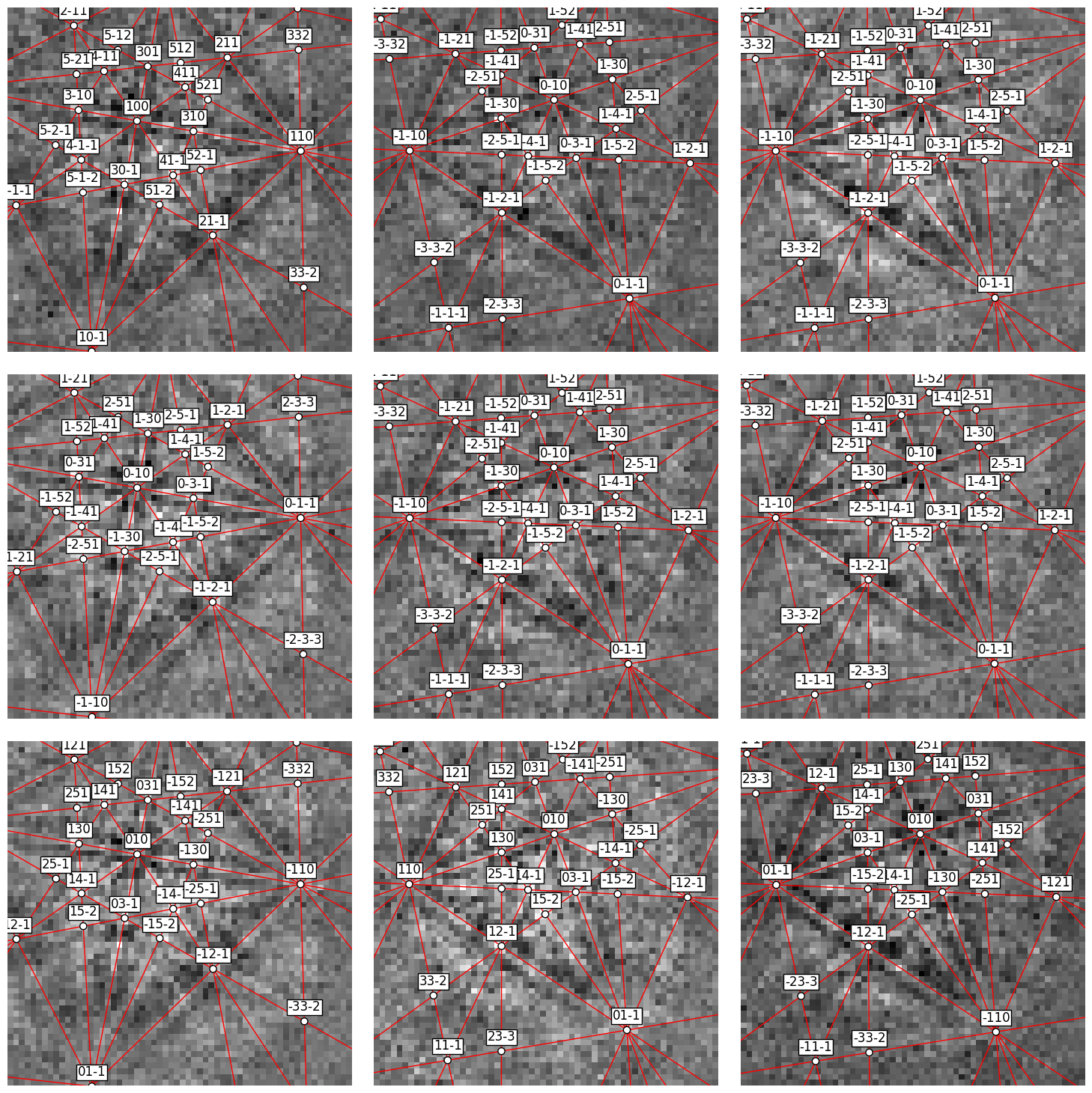
[22]:
fig, ax = plt.subplots(ncols=3, nrows=3, figsize=(15, 15))

for idx in np.ndindex(s.axes_manager.navigation_shape[::-1]):
    ax[idx].imshow(s.data[idx], cmap="gray")
    ax[idx].axis("off")

    lines, zone_axes, zone_axes_labels = sim.as_collections(
        idx,
        zone_axes=True,
        zone_axes_labels=True,
        zone_axes_labels_kwargs=dict(fontsize=12),
    )
    ax[idx].add_collection(lines)
    ax[idx].add_collection(zone_axes)
    for label in zone_axes_labels:
        ax[idx].add_artist(label)

fig.tight_layout()
Or, we can obtain the lines, zone axes, zone axes labels and PCs as HyperSpy markers via GeometricalKikuchiPatternSimulation.as_markers() and add them to a signal of the same navigation shape as the simulation instance. This enables navigating the patterns with the geometrical simulations
[23]:
markers = sim.as_markers()

# To delete previously added permanent markers, do
# del s.metadata.Markers

s.add_marker(markers, plot_marker=False, permanent=True)
[24]:
s.plot()