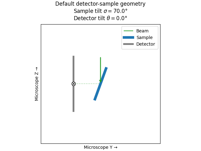
Detector-sample geometry views

This example shows how to plot multiple views of the detector-sample geometry in a single figure using the EBSDDetector. Both a side view and top view are available.

These can be useful when demonstrating variations in geometry parameters in a single figure.

For a more in-depth tutorial on the various reference frames in kikuchipy, see the reference frames tutorial.

Note

The side view shows changes to the following geometry parameters:

• tilt

• sample_tilt

• pcy

• pcz

The top view shows changes to the following geometry parameters:

• sample_tilt

• tilt

• azimuthal

• pcx

• pcy

• pcz

None of these views show changes in the detector twist angle.

Note

Use EBSDDetectorPlotter for a plot where all detector-sample geometry parameters can be changed interactively.

Imports and some reusable functions.

import matplotlib.pyplot as plt

import kikuchipy as kp


def tilt_string(detector: kp.detectors.EBSDDetector, fmt: str = "short") -> str:
    if fmt == "long":
        return (
            rf"Sample tilt $\sigma = {detector.sample_tilt:.1f}$"
            "\N{DEGREE SIGN}\n"
            rf"Detector tilt $\theta = {detector.tilt:.1f}$"
            "\N{DEGREE SIGN}"
        )
    else:
        return (
            r"($\sigma$, $\theta$) = "
            f"({detector.sample_tilt:.1f}"
            "\N{DEGREE SIGN}, "
            f"{detector.tilt:.1f}"
            "\N{DEGREE SIGN})"
        )


def pc_string(detector: kp.detectors.EBSDDetector) -> str:
    pcx, pcy, pcz = detector.pc_average.round(2)
    return f"(PCx, PCy, PCz) = ({pcx}, {pcy}, {pcz})"

Get the default detector with a rectangular shape.

shape = (75, 100)
det1 = kp.detectors.EBSDDetector(shape)
print(det1)

EBSDDetector
  shape (Ny, Nx):     (75, 100)
  pc (PCx, PCy, PCz): (0.5, 0.5, 0.5)
  sample_tilt:        70.0°
  tilt:               0.0°
  azimuthal:          0.0°
  twist:              0.0°
  binning:            1
  px_size:            1.0 um

And view the detector-sample geometry.

fig = det1.plot_side_view(legend=True, return_figure=True)
_ = fig.suptitle(f"Default detector-sample geometry\n{tilt_string(det1, fmt='long')}")

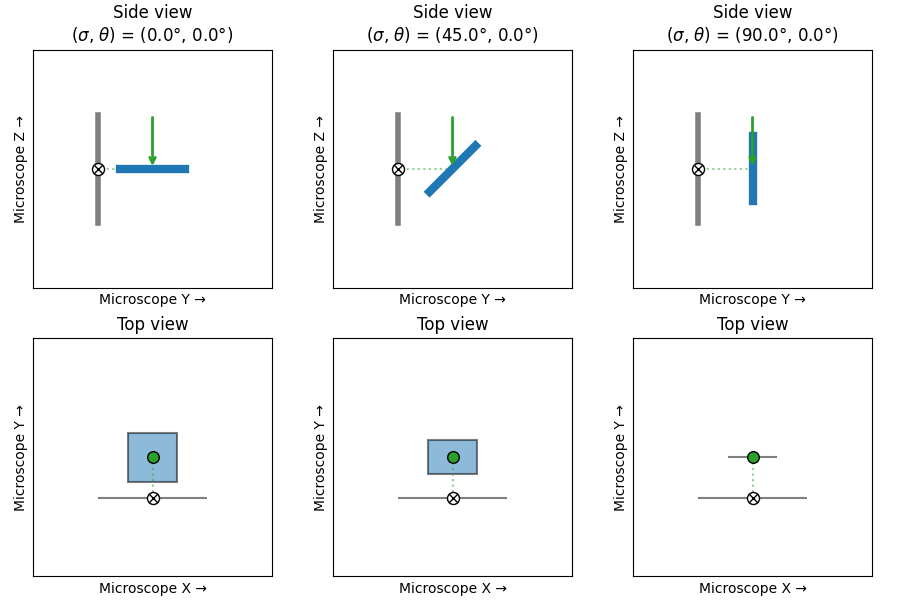
Changing sample tilt

det2 = kp.detectors.EBSDDetector(shape)

fig = plt.figure(figsize=(9, 6), layout="constrained")
for i, stilt in enumerate([0, 45, 90]):
    det2.sample_tilt = stilt

    ax1 = fig.add_subplot(2, 3, i + 1)
    ax1.set_title("Side view\n" + tilt_string(det2))
    det2.plot_side_view(ax=ax1)

    ax2 = fig.add_subplot(2, 3, i + 4)
    ax2.set_title("Top view")
    det2.plot_top_view(ax=ax2)

Changing detector tilt

det3 = kp.detectors.EBSDDetector(shape)

fig = plt.figure(figsize=(9, 6), layout="constrained")
for i, tilt in enumerate([0, 45, 90]):
    det3.tilt = tilt

    ax1 = fig.add_subplot(2, 3, i + 1)
    ax1.set_title("Side view\n" + tilt_string(det3))
    det3.plot_side_view(ax=ax1)

    ax2 = fig.add_subplot(2, 3, i + 4)
    ax2.set_title("Top view")
    det3.plot_top_view(ax=ax2)

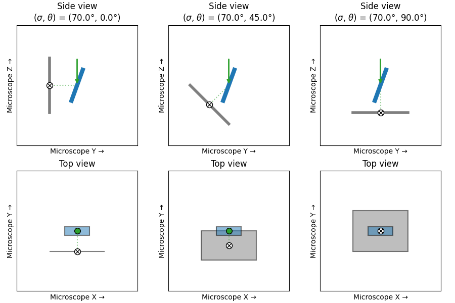
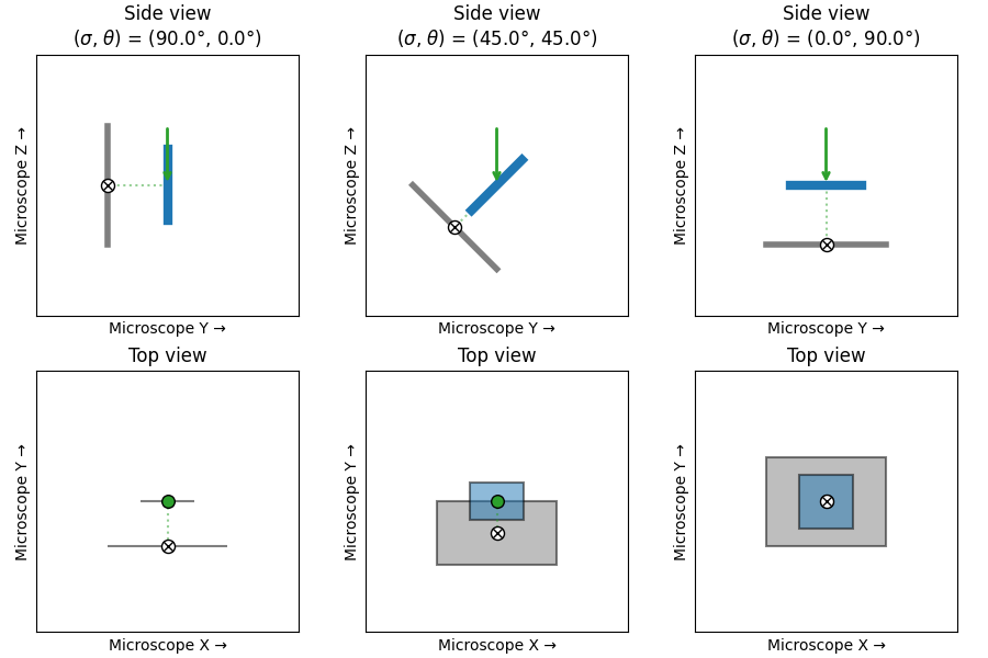
Changing sample and detector tilts

Let’s start with the sample tilt at \(\sigma = 90^{\circ}\) and then decrease it while increasing the detector tilt \(\theta\) in steps of \(10^{\circ}\).

det4 = kp.detectors.EBSDDetector(shape)

sample_tilts = [90, 45, 0]
detector_tilts = sample_tilts[::-1]

fig = plt.figure(figsize=(9, 6), layout="constrained")
for i, (stilt, tilt) in enumerate(zip(sample_tilts, detector_tilts)):
    det4.sample_tilt = stilt
    det4.tilt = tilt

    ax1 = fig.add_subplot(2, 3, i + 1)
    ax1.set_title("Side view\n" + tilt_string(det4))
    det4.plot_side_view(ax=ax1)

    ax2 = fig.add_subplot(2, 3, i + 4)
    ax2.set_title("Top view")
    det4.plot_top_view(ax=ax2)

Changing projection center

See the documentation for the EBSDDetector for a definition of the projection center (PC).

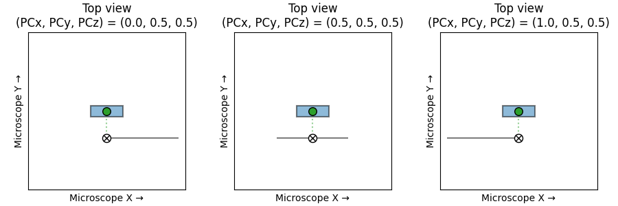
Changing PCx

Vary PCx from \(0 \rightarrow 1\) (left \(\rightarrow\) right).

det5 = kp.detectors.EBSDDetector(shape)

fig = plt.figure(figsize=(9, 3), layout="constrained")
for i, pcx in enumerate([0, 0.5, 1]):
    det5.pcx = pcx

    ax = fig.add_subplot(1, 3, i + 1)
    ax.set_title("Top view\n" + pc_string(det5))
    det5.plot_top_view(ax=ax)

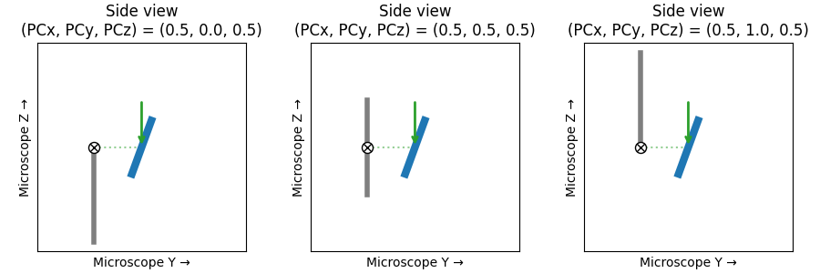
Changing PCy

Vary PCy from \(0 \rightarrow 1\) (top \(\rightarrow\) bottom).

det6 = kp.detectors.EBSDDetector(shape)

fig = plt.figure(figsize=(9, 3), layout="constrained")
for i, pcy in enumerate([0, 0.5, 1]):
    det6.pcy = pcy

    ax = fig.add_subplot(1, 3, i + 1)
    ax.set_title("Side view\n" + pc_string(det6))
    det6.plot_side_view(ax=ax)

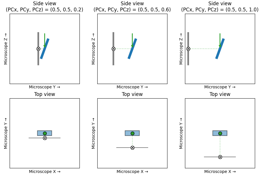
Changing PCz

Vary PCz from \(0.2 \rightarrow 1\) (increasing distance from the detector)

det7 = kp.detectors.EBSDDetector(shape)

fig = plt.figure(figsize=(9, 6), layout="constrained")
for i, pcz in enumerate([0.2, 0.6, 1]):
    det7.pcz = pcz

    ax1 = fig.add_subplot(2, 3, i + 1)
    ax1.set_title("Side view\n" + pc_string(det7))
    det7.plot_side_view(ax=ax1)

    ax2 = fig.add_subplot(2, 3, i + 4)
    ax2.set_title("Top view")
    det7.plot_top_view(ax=ax2)

Estimated memory usage: 790 MB