
Live notebook
You can run this notebook in a live session ![]() or view it on Github.
or view it on Github.
Kinematical EBSD simulations#
In this tutorial, we will perform kinematical Kikuchi pattern simulations of nickel, a variant of the \(\sigma\)-phase (Fe, Cr) in steels, and silicon carbide 6H.
We can generate kinematical master patterns using KikuchiPatternSimulator.calculate_master_pattern(). The simulator must be created from a ReciprocalLatticeVector instance that satisfy the following conditions:
All atom positions are filled in the unit cell, i.e. the
structureused to create thephaseused inReciprocalLatticeVector. This can be achieved by creating aPhaseinstance with all asymmetric atom positions listed, creating a reflector list, and then calling ReciprocalLatticeVector.sanitise_phase(). The phase can be created manually or imported from a valid CIF file with Phase.from_cif().The atoms in the
structurehave their elements described by the symbol (Ni), not by the atomic number (28).The lattice parameters \((a, b, c)\) are given in Ångström.
Kinematical structure factors \(F_{\mathrm{hkl}}\) have been calculated with ReciprocalLatticeVector.calculate_structure_factor().
Bragg angles \(\theta_{\mathrm{B}}\) have been calculated with ReciprocalLatticeVector.calculate_theta().
Let’s import the necessary libraries
[1]:
# Exchange inline for notebook or qt5 (from pyqt) for interactive plotting
%matplotlib inline

import matplotlib.pyplot as plt
import numpy as np
import pyvista as pv

from diffpy.structure import Atom, Lattice, Structure
from diffsims.crystallography import ReciprocalLatticeVector
import hyperspy.api as hs
import kikuchipy as kp
from orix.crystal_map import Phase

# Plotting parameters
plt.rcParams.update(
    {"figure.figsize": (10, 10), "font.size": 20, "lines.markersize": 10}
)
# See https://docs.pyvista.org/user-guide/jupyter/index.html
pv.set_jupyter_backend("static")
Nickel#
We’ll compare our kinematical simulations to dynamical simulations performed with EMsoft (see [Callahan and De Graef, 2013]), since we have a nickel master pattern available in the kikuchipy.data module
[2]:
mp_ni_dyn = kp.data.nickel_ebsd_master_pattern_small(
    projection="stereographic"
)
Inspect the phase
<name: ni. space group: Fm-3m. point group: m-3m. proper point group: 432. color: tab:blue>
Lattice(a=0.35236, b=0.35236, c=0.35236, alpha=90, beta=90, gamma=90)
Change lattice parameters from nm to Ångström
[4]:
lat_ni = phase_ni.structure.lattice  # Shallow copy
lat_ni.setLatPar(lat_ni.a * 10, lat_ni.b * 10, lat_ni.c * 10)

print(phase_ni.structure.lattice)
Lattice(a=3.5236, b=3.5236, c=3.5236, alpha=90, beta=90, gamma=90)
We’ll build up the reflector list by:
Finding all reflectors with a minimal interplanar spacing \(d\)
Keeping those that have a structure factor above a certain \(|F_{\mathrm{min}}|\) of the reflector with the highest structure factor \(|F_{\mathrm{max}}|\)
[5]:
ref_ni = ReciprocalLatticeVector.from_min_dspacing(phase_ni, 0.5)

# Exclude non-allowed reflectors (not available for hexagonal or trigonal
# phases!)
ref_ni = ref_ni[ref_ni.allowed]
ref_ni = ref_ni.unique(use_symmetry=True).symmetrise()
Sanitise the phase by completing the unit cell
[6]:
ref_ni.phase.structure
[6]:
[28 0.000000 0.000000 0.000000 1.0000]
[7]:
ref_ni.sanitise_phase()
ref_ni.phase.structure
[7]:
[Ni   0.000000 0.000000 0.000000 1.0000,
 Ni   0.000000 0.500000 0.500000 1.0000,
 Ni   0.500000 0.000000 0.500000 1.0000,
 Ni   0.500000 0.500000 0.000000 1.0000]
We can now calculate the structure factors \(F\). Two parametrizations are available, from [Kirkland, 1998] ("xtables", the default) and [Lobato and Van Dyck, 2014] ("lobato")
[8]:
ref_ni.calculate_structure_factor()
[9]:
F_ni = abs(ref_ni.structure_factor)
ref_ni = ref_ni[F_ni > 0.05 * F_ni.max()]

ref_ni.print_table()
 h k l      d     |F|_hkl   |F|^2   |F|^2_rel   Mult
 1 1 1    2.034    11.8     140.0     100.0      8
 2 0 0    1.762    10.4     108.2      77.3      6
 2 2 0    1.246     7.4     55.0       39.3      12
 3 1 1    1.062     6.2     38.6       27.6      24
 2 2 2    1.017     5.9     34.7       24.8      8
 4 0 0    0.881     4.9     23.9       17.1      6
 3 3 1    0.808     4.3     18.8       13.4      24
 4 2 0    0.788     4.2     17.4       12.5      24
 4 2 2    0.719     3.6     13.3       9.5       24
 5 1 1    0.678     3.3     11.1       8.0       24
 3 3 3    0.678     3.3     11.1       8.0       8
 4 4 0    0.623     2.9      8.6       6.1       12
 5 3 1    0.596     2.7      7.4       5.3       48
 6 0 0    0.587     2.7      7.1       5.1       6
 4 4 2    0.587     2.7      7.1       5.1       24
 6 2 0    0.557     2.4      6.0       4.3       24
 5 3 3    0.537     2.3      5.3       3.8       24
 6 2 2    0.531     2.3      5.1       3.7       24
 4 4 4    0.509     2.1      4.4       3.2       8
Calculate the Bragg angle \(\theta_{\mathrm{B}}\)
[10]:
ref_ni.calculate_theta(20e3)
We can now create our simulator and plot the simulation
[11]:
simulator_ni = kp.simulations.KikuchiPatternSimulator(ref_ni)
simulator_ni.reflectors.size
[11]:
338
Plotting the band centers with intensities scaled by the structure factor \(|F|\)
[12]:
simulator_ni.plot()
Or no scaling, \(|F|\) = 1 (scaling="square" for the structure factor squared \(|F|^2\))
[13]:
simulator_ni.plot(scaling=None)
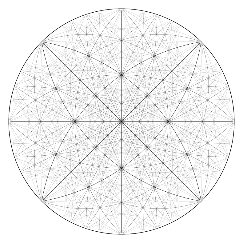
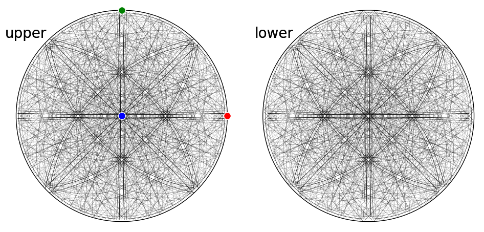
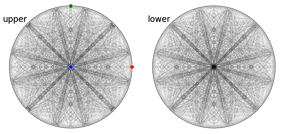
We can also plot the Kikuchi bands, showing both hemispheres, also adding the crystal axes alignment
[14]:
fig = simulator_ni.plot(hemisphere="both", mode="bands", return_figure=True)

ax = fig.axes[0]
ax.scatter(simulator_ni.phase.a_axis, c="r", ec="w")
ax.scatter(simulator_ni.phase.b_axis, c="g", ec="w")
ax.scatter(simulator_ni.phase.c_axis, c="b", ec="w")
fig.tight_layout()
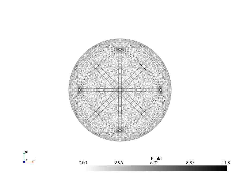
The simulation can be plotted in the spherical projection as well using Matplotlib or PyVista, provided that it is installed
[15]:
simulator_ni.plot("spherical", mode="bands")
[16]:
simulator_ni.plot("spherical", mode="bands", backend="pyvista")
2026-06-14 13:03:49.897 ( 5.381s) [ 7EF2948E6740]vtkXOpenGLRenderWindow.:1460 WARN| bad X server connection. DISPLAY=
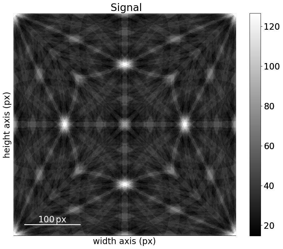
When we’re happy with the reflector list in the simulator, we can generate our kinematical master pattern
[17]:
mp_ni_kin = simulator_ni.calculate_master_pattern(half_size=200)
100%|█████████████████████████████████████████████| 1/1 [00:00<00:00, 5.36it/s]
The returned master pattern is an instance of EBSDMasterPattern in the stereographic projection
[18]:
[18]:
<EBSDMasterPattern, title: , dimensions: (|401, 401)>
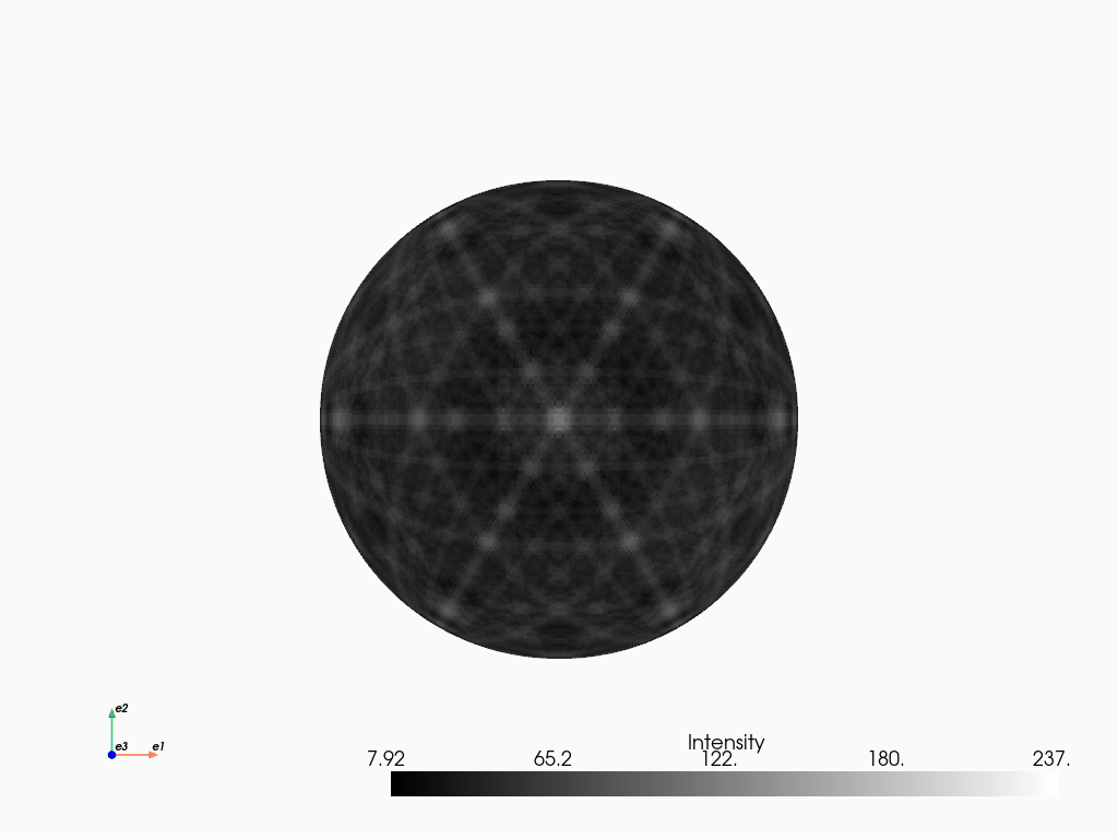
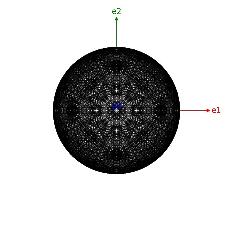
A spherical plot (requires that PyVista is installed)
[19]:
mp_ni_kin.plot_spherical(style="points")

Comparing kinematical and dynamical simulations
[20]:
# Exclude outside equator
ni_dyn_data = mp_ni_dyn.data.astype("float32")
ni_kin_data = mp_ni_kin.data.astype("float32")
mask = ni_dyn_data == 0
ni_dyn_data[mask] = np.nan
ni_kin_data[mask] = np.nan

fig, axes = plt.subplots(ncols=2, layout="tight")
for ax, data, title in zip(
    axes, [ni_kin_data, ni_dyn_data], ["kinematical", "dynamical"]
):
    ax.imshow(data, cmap="gray")
    ax.axis("off")
    ax.set(title=f"Ni {title} 20 kV")
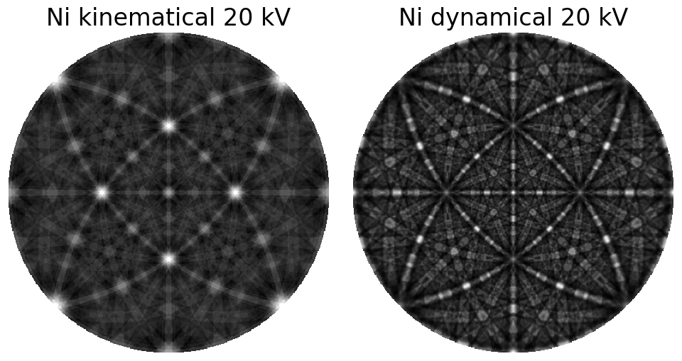
Warning
Use dynamical simulations when performing pattern matching, not kinematical simulations. The latter intensities are not realistic, as demonstrated in the above comparison.
Finally, we can transform the master pattern in the stereographic projection to one in the Lambert projection
[21]:
mp_ni_kin_lp = mp_ni_kin.as_lambert()
100%|██████████| 1/1 [00:00<00:00, 15.54it/s]
[22]:
mp_ni_kin_lp.plot()
We can then project parts of this pattern onto our EBSD detector using get_patterns(). Let’s do this for the (3, 3) patterns used to demonstrate geometrical simulations in the geometrical EBSD simulations tutorial. These patterns are stored with the indexed solutions and an optimized detector-sample geometry (both found using PyEBSDIndex, see the Hough indexing for details)
[23]:
s = kp.data.nickel_ebsd_small(lazy=True)  # Don't load the patterns

Gr = s.xmap.rotations
Gr = Gr.reshape(*s.xmap.shape)
print(Gr)

print(s.detector)
Rotation (3, 3)
[[[ 0.8743  0.0555  0.475   0.083 ]
  [ 0.4745  0.2915  0.4221 -0.7153]
  [ 0.4761  0.2915  0.4232 -0.7136]]

 [[ 0.2686 -0.1295  0.6879 -0.6618]
  [ 0.4755  0.2923  0.4244 -0.713 ]
  [ 0.4773  0.2925  0.4251 -0.7113]]

 [[ 0.5608 -0.2951  0.3731  0.6776]
  [ 0.7103 -0.4248  0.294   0.4781]
  [ 0.2999  0.0357  0.7124  0.6335]]]
EBSDDetector
  shape (Ny, Nx):     (60, 60)
  pc (PCx, PCy, PCz): (0.425, 0.213, 0.501)
  sample_tilt:        70.0°
  tilt:               0.0°
  azimuthal:          0.0°
  twist:              0.0°
  binning:            8
  px_size:            1.0 um
[24]:
s_kin = mp_ni_kin_lp.get_patterns(Gr, s.detector, energy=20, compute=True)
[########################################] | 100% Completed | 101.37 ms
[25]:
_ = hs.plot.plot_images(
    s_kin, axes_decor=None, label=None, colorbar=False, tight_layout=True
)
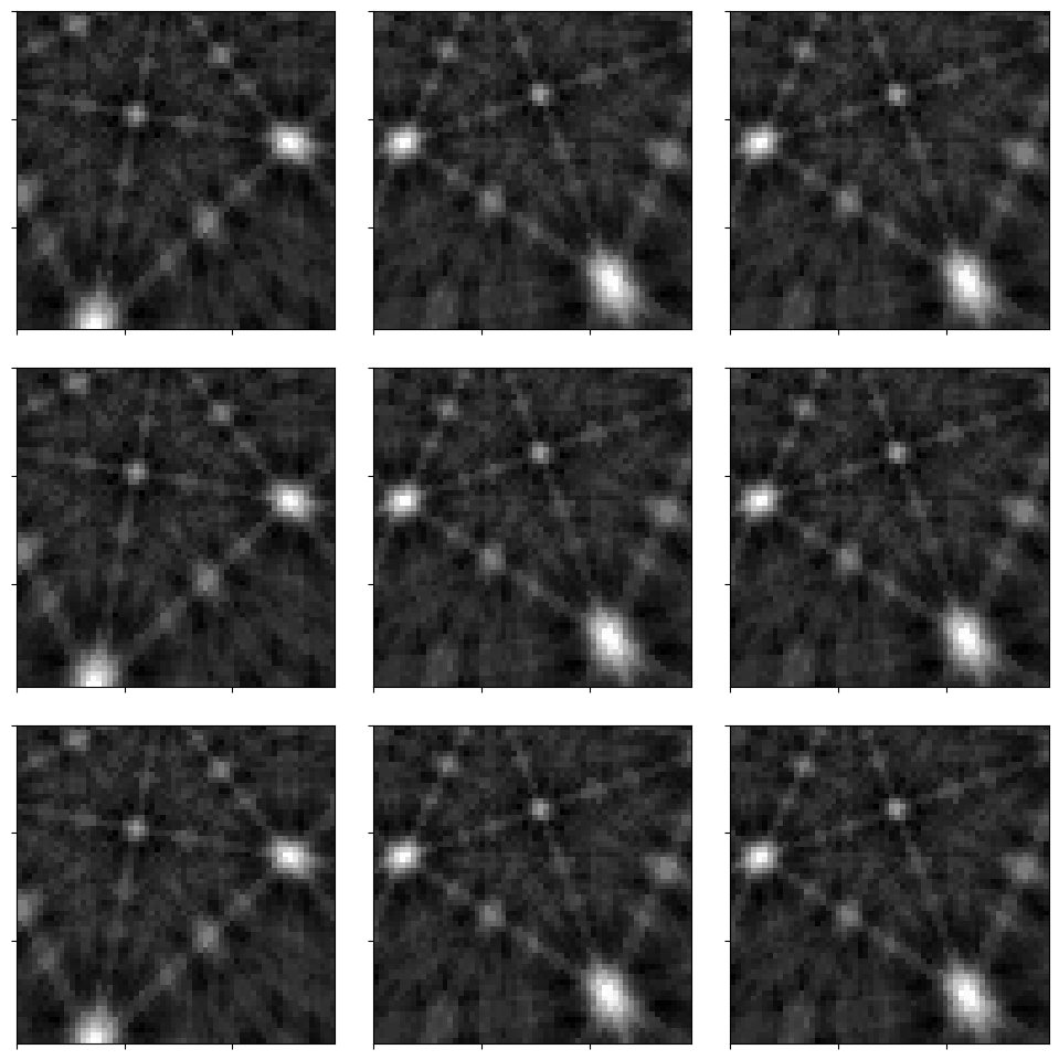
Feel free to compare these patterns to the experimental patterns in the geometrical EBSD simulations tutorial!
Sigma phase#
[26]:
phase_sigma = Phase(
    name="sigma",
    space_group=136,
    structure=Structure(
        atoms=[
            Atom("Cr", [0, 0, 0], 0.5),
            Atom("Fe", [0, 0, 0], 0.5),
            Atom("Cr", [0.31773, 0.31773, 0], 0.5),
            Atom("Fe", [0.31773, 0.31773, 0], 0.5),
            Atom("Cr", [0.06609, 0.26067, 0], 0.5),
            Atom("Fe", [0.06609, 0.26067, 0], 0.5),
            Atom("Cr", [0.13122, 0.53651, 0], 0.5),
            Atom("Fe", [0.13122, 0.53651, 0], 0.5),
        ],
        lattice=Lattice(8.802, 8.802, 4.548, 90, 90, 90),
    ),
)
phase_sigma
[26]:
<name: sigma. space group: P42/mnm. point group: 4/mmm. proper point group: 422. color: tab:blue>
[27]:
ref_sigma = ReciprocalLatticeVector.from_min_dspacing(phase_sigma, 1)

ref_sigma.sanitise_phase()

ref_sigma.calculate_structure_factor("lobato")

F_sigma = abs(ref_sigma.structure_factor)
ref_sigma = ref_sigma[F_sigma > 0.05 * F_sigma.max()]

ref_sigma.calculate_theta(20e3)

ref_sigma.print_table()
 h k l      d     |F|_hkl   |F|^2   |F|^2_rel   Mult
 0 0 2    2.274    143.1   20470.3    100.0      2
 0 0 4    1.137    70.5    4970.7      24.3      2
 3 3 0    2.075    66.2    4381.5      21.4      4
 4 1 0    2.135    64.6    4170.3      20.4      8
 4 1 1    1.932    63.5    4027.8      19.7      16
 3 3 1    1.888    56.4    3185.6      15.6      8
 3 3 2    1.533    49.6    2461.7      12.0      8
 1 1 1    3.672    48.6    2361.2      11.5      8
 4 1 2    1.556    48.0    2299.3      11.2      16
 5 5 1    1.201    47.3    2232.9      10.9      8
 8 2 0    1.067    42.1    1775.5      8.7       8
 5 0 1    1.642    41.1    1688.5      8.2       8
 4 1 3    1.236    40.0    1599.1      7.8       16
 1 1 0    6.224    37.3    1391.3      6.8       4
 7 2 0    1.209    36.6    1337.2      6.5       8
 2 2 1    2.568    36.0    1297.3      6.3       8
 3 3 3    1.224    35.9    1290.3      6.3       8
 7 2 1    1.168    32.4    1048.0      5.1       16
 7 2 2    1.068    31.3     977.7      4.8       16
 6 6 0    1.037    31.3     977.4      4.8       4
 5 5 0    1.245    28.6     816.9      4.0       4
 4 1 4    1.004    28.5     814.4      4.0       16
 5 0 3    1.149    27.7     764.7      3.7       8
 3 2 0    2.441    27.4     748.8      3.7       8
 1 0 1    4.041    25.4     642.9      3.1       8
 5 5 2    1.092    24.3     590.9      2.9       8
 3 2 1    2.151    23.7     561.8      2.7       16
 6 4 1    1.179    22.9     522.5      2.6       16
 6 6 1    1.011    22.8     520.7      2.5       8
 1 1 3    1.473    22.5     504.7      2.5       8
 4 0 0    2.201    21.8     476.3      2.3       4
 4 4 1    1.472    21.8     475.6      2.3       8
 7 3 1    1.120    21.0     439.9      2.1       16
 2 2 3    1.363    19.9     394.7      1.9       8
 3 2 2    1.664    19.4     375.4      1.8       16
 8 2 1    1.039    19.3     374.0      1.8       16
 1 1 2    2.136    19.1     364.2      1.8       8
 4 3 1    1.642    18.3     336.3      1.6       16
 2 2 0    3.112    18.1     327.6      1.6       4
 5 1 0    1.726    17.1     292.8      1.4       8
 2 1 1    2.976    16.3     265.8      1.3       16
 4 0 2    1.581    16.0     257.3      1.3       8
 4 4 0    1.556    15.7     245.6      1.2       4
 3 1 0    2.783    15.5     241.3      1.2       8
 5 2 1    1.538    15.4     236.3      1.2       16
 4 4 3    1.086    15.3     233.2      1.1       8
 6 1 0    1.447    15.0     223.5      1.1       8
 7 0 1    1.212    14.5     211.4      1.0       8
 3 2 3    1.288    14.2     202.8      1.0       16
 2 0 0    4.401    14.2     202.6      1.0       4
 5 1 2    1.375    13.5     183.3      0.9       16
 8 3 0    1.030    12.8     164.7      0.8       8
 4 4 2    1.284    12.7     161.9      0.8       8
 4 3 3    1.149    12.3     152.3      0.7       16
 6 1 2    1.221    12.3     152.2      0.7       16
 6 1 1    1.379    11.7     136.8      0.7       16
 3 0 1    2.465    11.7     136.0      0.7       8
 2 2 2    1.836    11.7     135.9      0.7       8
 1 0 3    1.494    11.2     126.0      0.6       8
 3 2 4    1.031    11.2     125.0      0.6       16
 5 2 3    1.112    10.6     112.3      0.5       16
 3 1 2    1.761    10.5     109.4      0.5       16
 1 1 4    1.118     9.7     94.6       0.5       8
 8 3 1    1.005     9.6     91.2       0.4       16
 4 0 4    1.010     9.5     89.8       0.4       8
 6 2 1    1.331     9.2     84.6       0.4       16
 4 2 0    1.968     9.0     81.0       0.4       8
 4 3 0    1.760     8.7     75.7       0.4       8
 3 1 1    2.374     8.7     75.0       0.4       16
 6 1 3    1.047     8.4     70.2       0.3       16
 2 1 3    1.415     8.4     69.8       0.3       16
 2 0 2    2.020     8.0     64.7       0.3       8
 8 1 1    1.062     7.6     57.7       0.3       16
 6 5 0    1.127     7.5     56.6       0.3       8
 6 3 1    1.261     7.4     55.4       0.3       16
[28]:
[28]:
KikuchiPatternSimulator:
ReciprocalLatticeVector (788,), sigma (4/mmm)
[[ 8.  3.  1.]
 [ 8.  3.  0.]
 [ 8.  3. -1.]
 ...
 [-8. -3.  1.]
 [-8. -3.  0.]
 [-8. -3. -1.]]
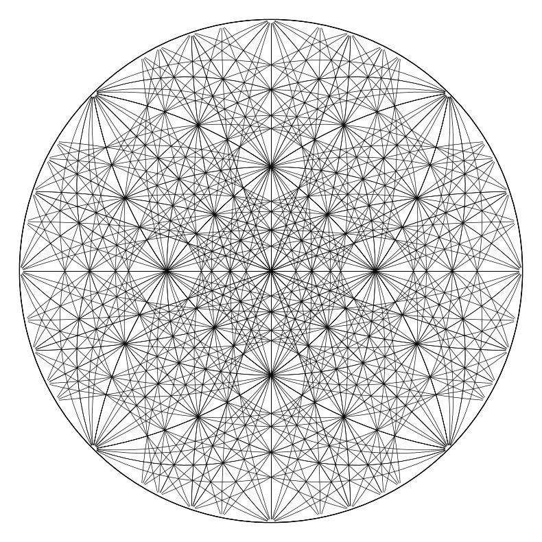
[29]:
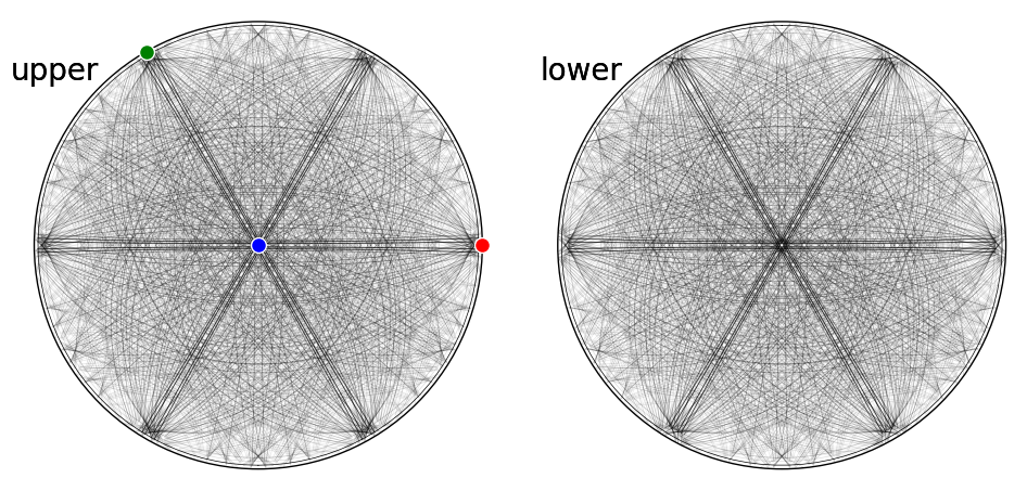
fig = simulator_sigma.plot(
    hemisphere="both", mode="bands", return_figure=True
)

ax = fig.axes[0]
ax.scatter(simulator_sigma.phase.a_axis, c="r", ec="w")
ax.scatter(simulator_sigma.phase.b_axis, c="g", ec="w")
ax.scatter(simulator_sigma.phase.c_axis, c="b", ec="w")
fig.tight_layout()
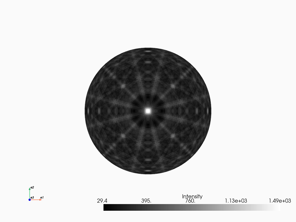
[30]:
simulator_sigma.plot("spherical", mode="bands", backend="pyvista")

[31]:
mp_sigma = simulator_sigma.calculate_master_pattern()
100%|█████████████████████████████████████████████| 1/1 [00:02<00:00, 2.64s/it]
[32]:
mp_sigma.plot()
[33]:
mp_sigma.plot_spherical(style="points")
Silicon carbide 6H#
[34]:
phase_sic = Phase(
    name="sic_6h",
    space_group=186,
    structure=Structure(
        atoms=[
            Atom("Si", [1 / 3, 2 / 3, 0.20778]),
            Atom("C", [1 / 3, 2 / 3, 0.33298]),
            Atom("Si", [1 / 3, 2 / 3, 0.54134]),
            Atom("C", [1 / 3, 2 / 3, 0.66647]),
            Atom("C", [0, 0, 0]),
            Atom("Si", [0, 0, 0.37461]),
        ],
        lattice=Lattice(3.081, 3.081, 15.2101, 90, 90, 120),
    ),
)
phase_sic
[34]:
<name: sic_6h. space group: P63mc. point group: 6mm. proper point group: 6. color: tab:blue>
[35]:
 h k l      d     |F|_hkl   |F|^2   |F|^2_rel   Mult
0   0   6  2.535    78.5    6161.5     100.0      1
0   0  -6  2.535    78.5    6161.5     100.0      1
0   0  -2  7.605    56.8    3226.1      52.4      1
0   0   2  7.605    56.8    3226.1      52.4      1
2  -1   0  1.541    37.8    1432.0      23.2      6
0   0  -8  1.901    29.8     887.9      14.4      1
0   0   8  1.901    29.8     887.9      14.4      1
2  -1   6  1.316    21.9     479.1      7.8       6
2  -1  -6  1.316    21.9     479.1      7.8       6
0   0   4  3.803    18.6     347.5      5.6       1
0   0  -4  3.803    18.6     347.5      5.6       1
0   0 -18  0.845    17.2     295.8      4.8       1
0   0  18  0.845    17.2     295.8      4.8       1
0   0  10  1.521    15.5     241.8      3.9       1
0   0 -10  1.521    15.5     241.8      3.9       1
0   0 -12  1.268    10.8     116.1      1.9       1
0   0  12  1.268    10.8     116.1      1.9       1
0   0  16  0.951    10.5     110.0      1.8       1
0   0 -16  0.951    10.5     110.0      1.8       1
2   0   0  1.334    10.4     108.6      1.8       6
2  -1   9  1.138    10.4     107.2      1.7       6
2  -1  -9  1.138    10.4     107.2      1.7       6
1   0   0  2.668     9.9     97.9       1.6       6
0   0 -14  1.086     9.8     96.1       1.6       1
0   0  14  1.086     9.8     96.1       1.6       1
2  -1  18  0.741     9.3     86.7       1.4       6
2  -1 -18  0.741     9.3     86.7       1.4       6
2  -1   2  1.510     8.7     75.8       1.2       6
2  -1  -2  1.510     8.7     75.8       1.2       6
2  -1  -8  1.197     8.5     72.4       1.2       6
2  -1   8  1.197     8.5     72.4       1.2       6
2  -1  -1  1.533     8.1     65.6       1.1       6
2  -1   1  1.533     8.1     65.6       1.1       6
2   0   8  1.092     7.4     55.4       0.9       6
2   0  -8  1.092     7.4     55.2       0.9       6
2  -1   3  1.474     7.3     53.5       0.9       6
2  -1  -3  1.474     7.3     53.5       0.9       6
2   0   2  1.314     7.1     51.0       0.8       6
2   0  -2  1.314     7.1     50.9       0.8       6
2  -1 -15  0.847     6.7     44.9       0.7       6
2  -1  15  0.847     6.7     44.9       0.7       6
3   1   0  0.740     6.5     42.6       0.7       12
2   0  -6  1.181     6.3     40.1       0.7       6
2   0   6  1.181     6.3     40.0       0.6       6
2  -1   7  1.257     6.0     35.8       0.6       6
2  -1  -7  1.257     6.0     35.8       0.6       6
3  -1   0  1.008     6.0     35.5       0.6       12
1   0  -1  2.628     5.9     34.7       0.6       6
1   0   1  2.628     5.9     34.7       0.6       6
1   0   2  2.518     5.8     33.6       0.5       6
1   0  -2  2.518     5.8     33.6       0.5       6
2  -1 -12  0.979     5.5     30.3       0.5       6
2  -1  12  0.979     5.5     30.3       0.5       6
3   0   0  0.889     5.5     30.2       0.5       12
1   0   9  1.428     5.5     29.9       0.5       6
1   0  -9  1.428     5.5     29.9       0.5       6
2  -1  10  1.082     5.2     27.0       0.4       6
2  -1 -10  1.082     5.2     27.0       0.4       6
1   0   3  2.361     5.2     26.9       0.4       6
1   0  -3  2.361     5.2     26.9       0.4       6
2   2  -9  0.701     5.0     24.7       0.4       10
2   2   9  0.701     5.0     24.7       0.4       10
1   0  -6  1.838     4.8     22.6       0.4       6
1   0   6  1.838     4.7     22.5       0.4       6
2   0  10  1.003     4.7     22.3       0.4       6
2   0 -10  1.003     4.7     22.2       0.4       6
3   1   6  0.710     4.6     21.2       0.3       12
3   1  -6  0.710     4.6     21.1       0.3       12
2   0   9  1.047     4.6     20.9       0.3       6
2   0  -9  1.047     4.6     20.9       0.3       6
2  -1  16  0.809     4.6     20.7       0.3       6
2  -1 -16  0.809     4.6     20.7       0.3       6
2   0  16  0.774     4.4     19.0       0.3       6
2   0 -16  0.774     4.3     18.9       0.3       6
1   0   8  1.548     4.3     18.8       0.3       6
1   0  -8  1.548     4.3     18.7       0.3       6
2  -1  14  0.888     4.1     16.6       0.3       6
2  -1 -14  0.888     4.1     16.6       0.3       6
3   1  -2  0.737     4.0     15.8       0.3       12
3   1   2  0.737     4.0     15.8       0.3       12
3  -1   6  0.937     4.0     15.7       0.3       12
3  -1  -6  0.937     3.9     15.6       0.3       12
[36]:
[36]:
KikuchiPatternSimulator:
ReciprocalLatticeVector (402,), sic_6h (6mm)
[[ 3.  1.  6.]
 [ 3.  1.  2.]
 [ 3.  1.  0.]
 ...
 [-3. -1.  0.]
 [-3. -1. -2.]
 [-3. -1. -6.]]
[37]:
fig = simulator_sic.plot(hemisphere="both", mode="bands", return_figure=True)

ax = fig.axes[0]
ax.scatter(simulator_sic.phase.a_axis, c="r", ec="w")
ax.scatter(simulator_sic.phase.b_axis, c="g", ec="w")
ax.scatter(simulator_sic.phase.c_axis, c="b", ec="w")
fig.tight_layout()
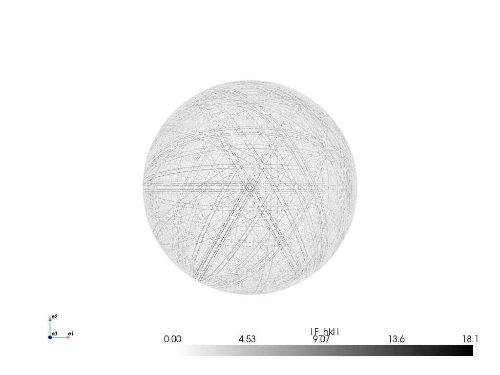
[38]:
simulator_sic.plot("spherical", mode="bands", backend="pyvista")
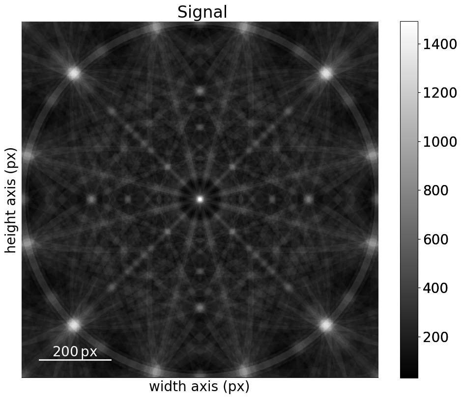
[39]:
mp_sic = simulator_sic.calculate_master_pattern(
    hemisphere="both", half_size=200
)
100%|█████████████████████████████████████████████| 2/2 [00:00<00:00, 4.54it/s]
[40]:
[40]:
<EBSDMasterPattern, title: , dimensions: (2|401, 401)>
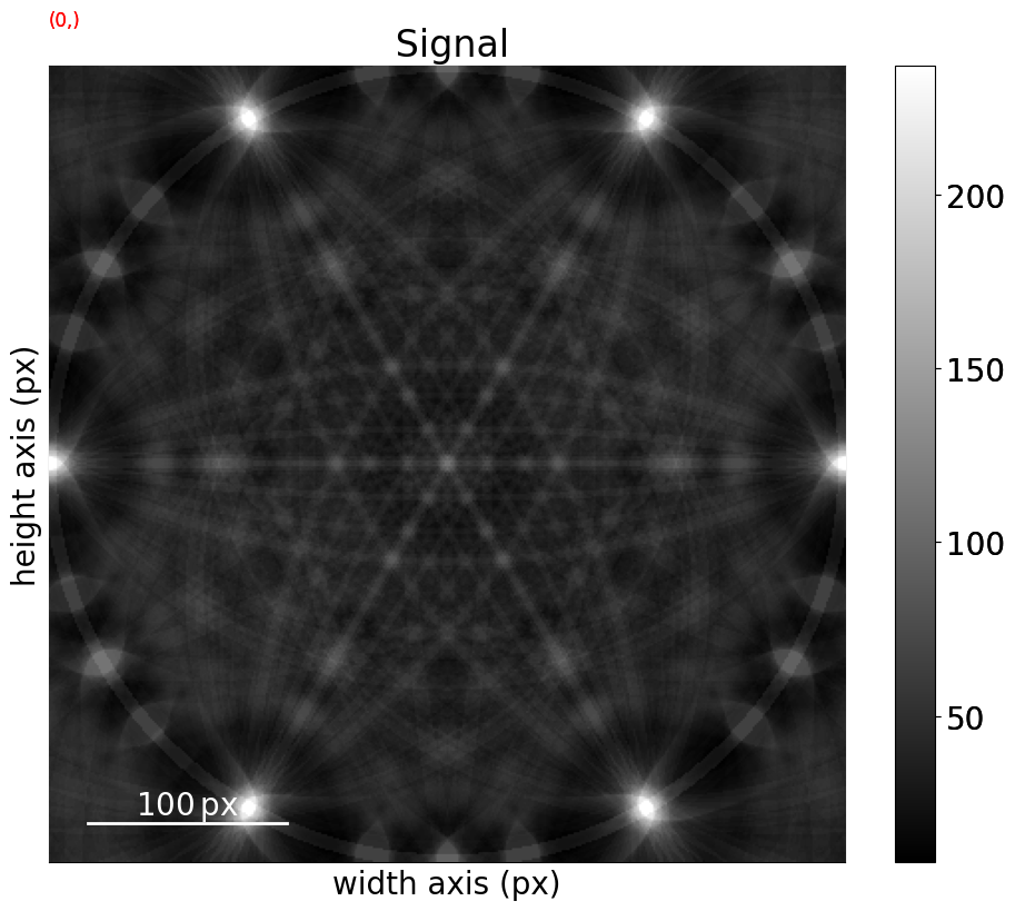
[41]:
mp_sic.plot(navigator=None)
[42]:
mp_sic.plot_spherical(style="points")