Live notebook

You can run this notebook in a live session or view it on Github.

Load and save data

In this tutorial, we will load and save electron backscatter diffraction (EBSD) patterns, Kikuchi master patterns generated with EMsoft and virtual backscatter electron (VBSE) images from and to various formats supported by kikuchipy.

Load patterns

From a file

kikuchipy can read and write experimental EBSD patterns and Kikuchi master patterns from or to many formats (see supported formats). To load patterns from a file use, the load() function. Let’s import the necessary libraries and read the nickel EBSD example dataset directly from file (not via kikuchipy.data.nickel_ebsd_small())

# Exchange inline for notebook or qt5 (from pyqt) for interactive plotting
%matplotlib inline

import os
from pathlib import Path
import tempfile

import dask.array as da
import imageio.v3 as iio
import numpy as np
import matplotlib.pyplot as plt

import hyperspy.api as hs
import kikuchipy as kp

datadir = Path("../../kikuchipy/data")
nordif_ebsd = "nordif/Pattern.dat"
s = kp.load(datadir / nordif_ebsd)
s

<EBSD, title: Pattern, dimensions: (3, 3|60, 60)>

Or, load the stereographic projection of the upper hemisphere of an EBSD master pattern for a 20 keV beam energy from a modified version of EMsoft’s master pattern file, returned from their EMEBSDmaster.f90 program

emsoft_master_pattern = (
    "emsoft_ebsd_master_pattern/ni_mc_mp_20kv_uint8_gzip_opts9.h5"
)
s_mp = kp.load(datadir / emsoft_master_pattern)
s_mp

<EBSDMasterPattern, title: ni_mc_mp_20kv_uint8_gzip_opts9, dimensions: (|401, 401)>

Both the stereographic and the square Lambert projections of this master pattern can be loaded with kikuchipy.data.nickel_ebsd_master_pattern_small().

All file readers support accessing the data’s metadata without loading it into memory (with the Dask library), which can be useful when processing large data sets, one data chunk at a time, to avoid memory errors

s_lazy = kp.load(datadir / nordif_ebsd, lazy=True)
print(s_lazy)
s_lazy.data

<LazyEBSD, title: Pattern, dimensions: (3, 3|60, 60)>

Array Chunk Bytes 31.64 kiB 31.64 kiB Shape (3, 3, 60, 60) (3, 3, 60, 60) Dask graph 1 chunks in 2 graph layers Data type uint8 numpy.ndarray

Parts or all of the data can be read into memory by calling compute()

s_lazy_copy = s_lazy.inav[:2, :].deepcopy()
s_lazy_copy.compute()
s_lazy_copy

[########################################] | 100% Completed | 102.17 ms

<EBSD, title: Pattern, dimensions: (2, 3|60, 60)>

s_lazy.compute()
s_lazy

[########################################] | 100% Completed | 101.59 ms

<EBSD, title: Pattern, dimensions: (3, 3|60, 60)>

Note

When lazily loaded EBSD patterns are processed, they are processed chunk by chunk, which can lead to longer processing times, so processing lazy data sets should be done with some care. See the relevant HyperSpy user guide for some tips.

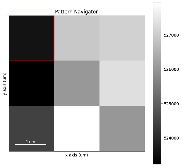
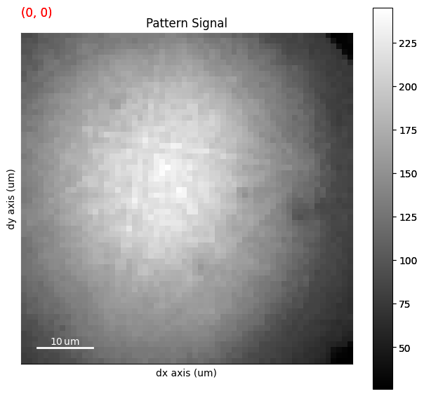
Patterns can be visualized by navigating the navigation space

s.plot()

Upon loading, kikuchipy reads some scan information from the file and stores it in the original_metadata attribute

# s.original_metadata  # Long output

Other information is stored in a standard location in the metadata attribute in fields specified in the HyperSpy metadata structure; these are not used by methods in kikuchipy

s.metadata

Acquisition_instrument
SEM
• beam_energy = 20.0
• magnification = 200
• microscope = Hitachi SU-6600
• working_distance = 24.7

General
• original_filename = ../../kikuchipy/data/nordif/Pattern.dat
• title = Pattern

Signal
• signal_type = EBSD

The number of patterns in horizontal and vertical direction, pattern size in pixels, scan step size and detector pixel size are stored in the axes_manager attribute

print(s.axes_manager)

<Axes manager, axes: (3, 3|60, 60)>
            Name |   size |  index |  offset |   scale |  units
================ | ====== | ====== | ======= | ======= | ======
               x |      3 |      0 |       0 |     1.5 |     um
               y |      3 |      0 |       0 |     1.5 |     um
---------------- | ------ | ------ | ------- | ------- | ------
              dx |     60 |      0 |       0 |       1 |     um
              dy |     60 |      0 |       0 |       1 |     um

This information can be modified directly, and information in metadata and axes_manager can be modified by the EBSD class methods set_scan_calibration() and set_detector_calibration().

In addition to the metadata, original_metadata and axes_manager properties, kikuchipy tries to read the following from the file if available:

• a CrystalMap with indexing results into the xmap attribute

• an EBSDDetector describing the projection/pattern center (PC) values into the detector attribute

• a static background into the static_background attribute.

The xmap attribute is None if it is not read, while some readers return an “empty” crystal map with points containing the identity rotation and the same phase ID of an undefined phase with no point group set.

s.xmap

Phase  Orientations  Name  Space group  Point group  Proper point group     Color
    0    9 (100.0%)  None         None         None                None  tab:blue
Properties:
Scan unit: px

s.xmap.rotations

Rotation (9,)
[[1. 0. 0. 0.]
 [1. 0. 0. 0.]
 [1. 0. 0. 0.]
 [1. 0. 0. 0.]
 [1. 0. 0. 0.]
 [1. 0. 0. 0.]
 [1. 0. 0. 0.]
 [1. 0. 0. 0.]
 [1. 0. 0. 0.]]

s.xmap.phase_id

array([0, 0, 0, 0, 0, 0, 0, 0, 0])

s.detector

EBSDDetector (60, 60), px_size 1 um, binning 1, tilt 0.0, azimuthal 0.0, pc (0.5, 0.5, 0.5)

s.detector.pc

array([[0.5, 0.5, 0.5]])

s.static_background

array([[84, 87, 90, ..., 27, 29, 30],
       [87, 90, 93, ..., 27, 28, 30],
       [92, 94, 97, ..., 39, 28, 29],
       ...,
       [80, 82, 84, ..., 36, 30, 26],
       [79, 80, 82, ..., 28, 26, 26],
       [76, 78, 80, ..., 26, 26, 25]], dtype=uint8)

Note

New in version 0.8.

The EBSD class inherits all methods from HyperSpy’s Signal2D class. An effort is made to handle the mentioned attributes of xmap, detector and static_background when the navigation and/or signal dimensions are cropped, like when calling EBSD.inav[] or EBSD.isig[]. This handling is new, and so needs time and more tests to mature. It is considered experimental functionality.

From a NumPy array

An EBSD, EBSDMasterPattern or ECPMasterPattern (electron channeling pattern) signal can be created directly from a NumPy array. To create a data set of (60 x 60) pixel patterns in a (10 x 20) grid, i.e. 10 and 20 patterns in the horizontal and vertical scan directions respectively, of random intensities

s_np = kp.signals.EBSD(np.random.random((20, 10, 60, 60)))
s_np

<EBSD, title: , dimensions: (10, 20|60, 60)>

From a Dask array

When processing large data sets, it is useful to load data lazily with the Dask library. This can be done upon reading patterns from a file by setting lazy=True when using the load() function, or directly from a dask.array.Array

s_da = kp.signals.LazyEBSD(
    da.random.random((20, 10, 60, 60), chunks=(2, 10, 60, 60))
)
print(s_da)
s_da.data

<LazyEBSD, title: , dimensions: (10, 20|60, 60)>

Array Chunk Bytes 5.49 MiB 562.50 kiB Shape (20, 10, 60, 60) (2, 10, 60, 60) Dask graph 10 chunks in 1 graph layer Data type float64 numpy.ndarray

From a HyperSpy signal

HyperSpy provides the method set_signal_type() to change between BaseSignal subclasses, of which EBSD, EBSDMasterPattern, ECPMasterPattern and VirtualBSEImage are four. To get one of these signals from a HyperSpy Signal2D signal

s_hs = hs.signals.Signal2D(np.random.random((20, 10, 60, 60)))
s_hs

<Signal2D, title: , dimensions: (10, 20|60, 60)>

for signal_type in [
    "EBSD",
    "VirtualBSEImage",
    "ECPMasterPattern",
    "EBSDMasterPattern",
]:
    s_hs.set_signal_type(signal_type)
    print(s_hs)

<EBSD, title: , dimensions: (10, 20|60, 60)>
<VirtualBSEImage, title: , dimensions: (10, 20|60, 60)>
<ECPMasterPattern, title: , dimensions: (10, 20|60, 60)>
<EBSDMasterPattern, title: , dimensions: (10, 20|60, 60)>

Save patterns

To save signals to file, use the save() method. For example, to save an EBSD signal in an HDF5 file in our default h5ebsd format, with file name "patterns.h5"

temp_dir = Path(tempfile.mkdtemp())
s.save(temp_dir / "patterns")

Warning

If we want to overwrite an existing file:

s.save("patterns.h5", overwrite=True)

If we want to save patterns in NORDIF’s binary format instead

s.save(temp_dir / "patterns.dat")

WARNING:hyperspy.signal:The default iterpath will change in HyperSpy 2.0.

To save an EBSDMasterPattern to an HDF5 file, we use the save method inherited from HyperSpy to write to their HDF5 specification or zarr specification

s_hs.save(temp_dir / "master_pattern.hspy")
s_hs

<EBSDMasterPattern, title: , dimensions: (10, 20|60, 60)>

These master patterns can then be read into an EBSDMasterPattern signal again via HyperSpy’s load()

s_mp2 = hs.load(
    temp_dir / "master_pattern.hspy", signal_type="EBSDMasterPattern"
)
s_mp2

<EBSDMasterPattern, title: , dimensions: (10, 20|60, 60)>

Note

To save results from statistical decomposition (machine learning) of patterns to file see the section Saving and loading results in HyperSpy’s user guide. Note that the file extension .hspy or .zspy must be used upon saving, s.save('patterns.hspy'), as the default extension in kikuchipy, .h5, yields a kikuchipy h5ebsd file where the decomposition results aren’t saved. The saved patterns can then be reloaded using HyperSpy’s load() function passing the signal_type="EBSD" parameter as explained above.

Supported file formats

Currently, kikuchipy has readers and writers for the following formats:

Format	Read	Write
EMsoft simulated EBSD HDF5	Yes	No
EMsoft EBSD master pattern HDF5	Yes	No
EMsoft ECP master pattern HDF5	Yes	No
EMsoft TKD master pattern HDF5	Yes	No
kikuchipy h5ebsd	Yes	Yes
Bruker h5ebsd	Yes	No
EDAX h5ebsd	Yes	No
EDAX binary	Yes	No
NORDIF binary	Yes	Yes
NORDIF calibration patterns	Yes	No
Oxford Instruments binary	Yes	No
Oxford Instruments h5ebsd (H5OINA)	Yes	No
Directory of EBSD patterns	Yes	No

Note

If you want to process your patterns with kikuchipy, but use an unsupported EBSD vendor software, or if you want to write your processed patterns to a vendor format that does not support writing, please request this feature in our issue tracker.

EMsoft simulated EBSD HDF5

Dynamically simulated EBSD patterns returned by EMsoft’s EMEBSD.f90 program as HDF5 files can be read as an EBSD signal

emsoft_ebsd = "emsoft_ebsd/simulated_ebsd.h5"  # Dummy data set
s_sim = kp.load(datadir / emsoft_ebsd)
s_sim

<EBSD, title: simulated_ebsd, dimensions: (10|10, 10)>

Here, the EMsoft simulated EBSD file_reader() is called, which takes the optional argument scan_size. Passing scan_size=(2, 5) will reshape the pattern data shape from (10, 10, 10) to (2, 5, 10, 10)

s_sim2 = kp.load(datadir / emsoft_ebsd, scan_size=(2, 5))
print(s_sim2)
print(s_sim2.data.shape)

<EBSD, title: simulated_ebsd, dimensions: (5, 2|10, 10)>
(2, 5, 10, 10)

Simulated EBSD patterns can be written to the kikuchipy h5ebsd format, the NORDIF binary format, or to HDF5/zarr files using HyperSpy’s HDF5/zarr specifications as explained above.

EMsoft EBSD master pattern HDF5

Master patterns returned by EMsoft’s EMEBSDmaster.f90 program as HDF5 files can be read as an EBSDMasterPattern signal

s_mp = kp.load(datadir / emsoft_master_pattern)

print(s_mp)
print(s_mp.projection)
print(s_mp.hemisphere)
print(s_mp.phase)

<EBSDMasterPattern, title: ni_mc_mp_20kv_uint8_gzip_opts9, dimensions: (|401, 401)>
stereographic
upper
<name: ni. space group: Fm-3m. point group: m-3m. proper point group: 432. color: tab:blue>

Here, the EMsoft EBSD master pattern file_reader() is called, which takes the optional arguments projection, hemisphere and energy. The stereographic projection is read by default. Passing projection="lambert" will read the square Lambert projection instead. The upper hemisphere is read by default. Passing hemisphere="lower" or hemisphere="both" will read the lower hemisphere projection or both, respectively. Master patterns for all beam energies are read by default. Passing energy=(10, 20) or energy=15 will read the master pattern(s) with beam energies from 10 to 20 keV, or just 15 keV, respectively

s_mp = kp.load(
    datadir / emsoft_master_pattern,
    projection="lambert",
    hemisphere="both",
    energy=20,
)

print(s_mp)
print(s_mp.projection)
print(s_mp.hemisphere)

<EBSDMasterPattern, title: ni_mc_mp_20kv_uint8_gzip_opts9, dimensions: (2|401, 401)>
lambert
both

Master patterns can be written to HDF5/zarr files using HyperSpy’s HDF5/zarr specification as explained above.

See [Jackson et al., 2019] for a hands-on tutorial explaining how to simulate these patterns with EMsoft, and [Callahan and De Graef, 2013] for details of the underlying theory.

EMsoft ECP master pattern HDF5

Master patterns returned by EMsoft’s EMECPmaster.f90 program as HDF5 files can be read as an ECPMasterPattern signal

# Load a dummy pattern
s_mp = kp.load(datadir / "emsoft_ecp_master_pattern/ecp_master_pattern.h5")

print(s_mp)
print(s_mp.projection)
print(s_mp.hemisphere)
print(s_mp.phase)

<ECPMasterPattern, title: ecp_master_pattern, dimensions: (11|13, 13)>
stereographic
upper
<name: None. space group: I4/mcm. point group: 4/mmm. proper point group: 422. color: tab:blue>

Here, the EMsoft ECP master pattern file_reader() is called, which supports the same parameters as the EMsoft EBSD master pattern reader.

EMsoft TKD master pattern HDF5

Master patterns returned by EMsoft’s EMTKDmaster.f90 program as HDF5 files can be read as an EBSDMasterPattern signal

# Load a dummy pattern
s_mp = kp.load(datadir / "emsoft_tkd_master_pattern/tkd_master_pattern.h5")

print(s_mp)
print(s_mp.projection)
print(s_mp.hemisphere)
print(s_mp.phase)

<EBSDMasterPattern, title: tkd_master_pattern, dimensions: (11|13, 13)>
stereographic
upper
<name: None. space group: I4/mcm. point group: 4/mmm. proper point group: 422. color: tab:blue>

Here, the EMsoft TKD master pattern file_reader() is called, which supports the same parameters as the EMsoft EBSD master pattern reader.

kikuchipy h5ebsd

The h5ebsd format [Jackson et al., 2014] is based on the HDF5 open standard (Hierarchical Data Format version 5). HDF5 files can be read and edited using e.g. the HDF Group’s reader HDFView or the Python package h5py. Upon loading an HDF5 file with extension .h5, .hdf5, or .h5ebsd, the correct reader is determined from the file. Other supported h5ebsd formats are listed in the table above.

If an h5ebsd file contains multiple scans, as many scans as desirable can be read from the file. For example, if the file contains two scans with names "Scan 1" and "Scan 2"

kikuchipy_ebsd = "kikuchipy_h5ebsd/patterns.h5"
s1, s2 = kp.load(
    datadir / kikuchipy_ebsd, scan_group_names=["Scan 1", "Scan 2"]
)
print(s1)
print(s2)

<EBSD, title: patterns Scan 1, dimensions: (3, 3|60, 60)>
<EBSD, title: patterns Scan 2, dimensions: (3, 3|60, 60)>

Here, the h5ebsd file_reader() is called. If only "Scan 1" is to be read, scan_group_names="Scan 1" can be passed

s1 = kp.load(datadir / kikuchipy_ebsd, scan_group_names="Scan 1")
s1

<EBSD, title: patterns Scan 1, dimensions: (3, 3|60, 60)>

The scan_group_names parameter is unnecessary if only the first scan in the file is to be read, since reading only the first scan in the file is the default behaviour.

So far, only saving patterns to kikuchipy’s own h5ebsd format is supported. It is possible to write a new scan with a scan name "Scan x", where x is an integer, to an existing, but closed, h5ebsd file in the kikuchipy format, e.g. one containing only Scan 1, by passing

new_file = "patterns_new.h5"
s1.save(temp_dir / new_file, scan_number=1)
s2.save(temp_dir / new_file, add_scan=True, scan_number=2)

s1_new, s2_new = kp.load(
    temp_dir / new_file, scan_group_names=["Scan 1", "Scan 2"]
)
print(s1_new)
print(s2_new)

<EBSD, title: patterns_new Scan 1, dimensions: (3, 3|60, 60)>
<EBSD, title: patterns_new Scan 2, dimensions: (3, 3|60, 60)>

Here, the h5ebsd file_writer() is called. The EBSD class attributes xmap (crystal map), detector (EBSD detector) and static_background are written to and read from file if available.

Bruker h5ebsd

Bruker Nano’s h5ebsd files with extension .h5, .hdf5, or .h5ebsd can be read. Available parameters when calling kikuchipy.load("bruker_patterns.h5") are described in the file_reader(). As with the kikuchipy h5ebsd reader, multiple scans can be read at once.

The projection center (PC) arrays are read into the detector attribute, and the static background pattern is read into the static_background attribute. The orientation and phase data are so far not read, but note that this can be read using orix.

EDAX h5ebsd

EDAX’s h5ebsd files with extension .h5, .hdf5, or .h5ebsd can be read. Available parameters when calling kikuchipy.load("edax_patterns.h5") are described in the file_reader(). As with the kikuchipy h5ebsd reader, multiple scans can be read at once.

The projection center (PC) arrays are read into the detector attribute. The orientation and phase data are so far not read.

EDAX binary

Patterns stored in the EDAX TSL’s binary UP1/2 file format, with intensities as 8-bit or 16-bit unsigned integer, can be read. File version 1 and >= 3 are supported.

edax_binary_path = datadir / "edax_binary/"  # Directory with dummy signals
s_edax = kp.load(edax_binary_path / "edax_binary.up1")
s_edax

<EBSD, title: edax_binary, dimensions: (9|60, 60)>

Here, the EDAX binary file_reader() is called.

Files with version 1 has no information on the navigation (map) shape, so we can pass this to the reader in the nav_shape parameter

s_edax2 = kp.load(edax_binary_path / "edax_binary.up1", nav_shape=(3, 3))
s_edax2

<EBSD, title: edax_binary, dimensions: (3, 3|60, 60)>

Patterns acquired in an hexagonal grid can be read, but the returned signal will have only one navigation dimension

s_edax3 = kp.load(edax_binary_path / "edax_binary.up2")
s_edax3

/home/docs/checkouts/readthedocs.org/user_builds/kikuchipy/conda/stable/lib/python3.11/site-packages/kikuchipy/io/plugins/edax_binary.py:152: UserWarning: Returned signal has one navigation dimension since an hexagonal grid is not supported
  warnings.warn(

<EBSD, title: edax_binary, dimensions: (10|60, 60)>

NORDIF binary

Patterns acquired using NORDIF’s acquisition software are stored in a binary file usually named “Pattern.dat”. Scan information is stored in a separate text file usually named “Setting.txt”, and both files usually reside in the same directory. If this is the case, the patterns can be loaded by passing the file name as the only parameter. If this is not the case, the setting file can be passed upon loading

s_nordif = kp.load(
    datadir / nordif_ebsd, setting_file=datadir / "nordif/Setting.txt"
)
s_nordif

<EBSD, title: Pattern, dimensions: (3, 3|60, 60)>

Here, the NORDIF file_reader() is called. If the scan information, i.e. scan and pattern size, in the setting file is incorrect or the setting file is not available, patterns can be loaded by passing

s_nordif = kp.load(
    datadir / nordif_ebsd, scan_size=(1, 9), pattern_size=(60, 60)
)
s_nordif

<EBSD, title: Pattern, dimensions: (9|60, 60)>

If a static background pattern named “Background acquisition pattern.bmp” is stored in the same directory as the pattern file, this is stored in EBSD.static_background upon loading

s_nordif.static_background

array([[84, 87, 90, ..., 27, 29, 30],
       [87, 90, 93, ..., 27, 28, 30],
       [92, 94, 97, ..., 39, 28, 29],
       ...,
       [80, 82, 84, ..., 36, 30, 26],
       [79, 80, 82, ..., 28, 26, 26],
       [76, 78, 80, ..., 26, 26, 25]], dtype=uint8)

Patterns can also be saved to a NORDIF binary file, upon which the NORDIF file_writer() is called. Note, however, that so far no new setting file, background pattern, or calibration patterns are created upon saving.

NORDIF calibration patterns

NORDIF calibration patterns in bitmap format named “Calibration (x,y).bmp”, where “x” and “y” correspond to coordinates listed in the NORDIF setting file, usually named “Setting.txt”, can be loaded

s_nordif_cal = kp.load(datadir / "nordif/Setting.txt")
s_nordif_cal

<EBSD, title: Calibration patterns, dimensions: (2|60, 60)>

Here, the NORDIF calibration patterns file_reader() is called. Lazy loading is not supported for this reader, thus the lazy parameter is not used.

If a static background pattern named “Background calibration pattern.bmp” is stored in the same directory as the pattern file, this is stored in EBSD.static_background upon loading.

The pixel indices of the calibration patterns into the full electron image (named “Area.bmp” by the NORDIF software) are read into the original_metadata. The shapes of this image and the region of interest (ROI) of the scanned area within this image are also attempted to be read. All this information can be useful when obtaining a plane of projection centers (PCs) for all patterns in the full dataset based on these calibration patterns (see other user guide tutorials for this).

Oxford Instruments binary

Uncompressed patterns stored in the Oxford Instruments binary .ebsp file format, with intensities as 8-bit or 16-bit unsigned integer, can be read

oxford_binary_path = datadir / "oxford_binary"
s_oxford = kp.load(oxford_binary_path / "patterns.ebsp")
s_oxford

<EBSD, title: patterns, dimensions: (3, 3|60, 60)>

Here, the Oxford Instruments binary file_reader() is called.

Every pattern’s flattened index into the 2D navigation map, as well as their entry in the file (map order isn’t always the same as file order) can be retrieved from s_oxford.original_metadata.map1d_id and s_oxford.original_metadata.file_order, respectively. If available in the file, every pattern’s row and column beam position in microns can be retrieved from s_oxford.original_metadata.beam_y and s_oxford.original_metadata.beam_x, respectively. All these are 1D arrays.

s_oxford.original_metadata

• beam_x = array([0. , 1.5, 3. , 0. , 1.5, 3. , 0. , 1.5, 3. ])

• beam_y = array([0. , 0. , 0. , 1.5, 1.5, 1.5, 3. , 3. , 3. ])

• file_order = array([8, 0, 1, 2, 3, 4, 5, 6, 7])

• map1d_id = array([0, 1, 2, 3, 4, 5, 6, 7, 8])

If the beam positions aren’t present in the file, the returned signal will have a single navigation dimension the size of the number of patterns.

Files with only the non-indexed patterns can also be read. The returned signal will then have a single navigation dimension the size of the number of patterns. The flattened index into the 2D navigation map mentioned above can be useful to determine the location of each non-indexed pattern.

Oxford Instruments h5ebsd (H5OINA)

Oxford Instruments’ h5ebsd files (H5OINA) with extension .h5oina can be read. Available parameters when calling kikuchipy.load("patterns.h5oina") are described in the file_reader(). As with the kikuchipy h5ebsd reader, multiple scans can be read at once.

The projection center (PC) arrays are read into the detector attribute and the static background pattern is read into the static_background attribute. The orientation and phase data are so far not read.

Directory of EBSD patterns

Many EBSD patterns in image files in a directory can be read as an EBSD signal, assuming all images with that file extension have the same shape and data type. Valid formats are those supported by imageio.

To demonstrate how the images can be read, we will first write nine patterns to a temporary with their filenames formatted a certain way

temp_dir2 = Path(tempfile.mkdtemp())
s = kp.data.nickel_ebsd_small()
y, x = np.indices(s.axes_manager.navigation_shape[::-1])
y = y.ravel()
x = x.ravel()
s.unfold_navigation_space()
for i in range(s.axes_manager.navigation_size):
    iio.imwrite(temp_dir2 / f"pattern_x{x[i]}y{y[i]}.tif", s.data[i])

# Print file contents
os.listdir(temp_dir2)

['pattern_x1y1.tif',
 'pattern_x2y2.tif',
 'pattern_x0y0.tif',
 'pattern_x2y1.tif',
 'pattern_x0y2.tif',
 'pattern_x1y2.tif',
 'pattern_x0y1.tif',
 'pattern_x1y0.tif',
 'pattern_x2y0.tif']

If filenames are formatted like this _x0y0.tif or -0-0.png, we do not have to specify this file name pattern when reading the images

s1 = kp.load(temp_dir2 / "*.tif")
s1

<EBSD, title: , dimensions: (3, 3|60, 60)>

Here file_reader() of this plugin was called. If filenames are formatted some other way, we have to pass this as a regular expression to xy_pattern

s2 = kp.load(
    temp_dir2 / "*.tif",
    xy_pattern=r"_x(\d+)y(\d+).tif",
    show_progressbar=True,
)
s2

[########################################] | 100% Completed | 109.04 ms

<EBSD, title: , dimensions: (3, 3|60, 60)>

Here we also printed a progressbar when reading the patterns from file, which can be useful when we want to read a large number of images.

From kikuchipy into other software

Patterns saved in the h5ebsd format can be read by the dictionary indexing and related routines in EMsoft using the EMEBSD reader. Those routines in EMsoft also have a NORDIF reader.

Patterns saved in the h5ebsd format can of course be read in Python like any other HDF5 data set

import h5py

with h5py.File(datadir / kikuchipy_ebsd, mode="r") as f:
    dset = f["Scan 2/EBSD/Data/patterns"]
    print(dset)
    patterns = dset[()]
    print(patterns.shape)
    plt.figure()
    plt.imshow(patterns[0], cmap="gray")
    plt.axis("off")

<HDF5 dataset "patterns": shape (9, 60, 60), type "|u1">
(9, 60, 60)

Load and save virtual BSE images

One or more virtual backscatter electron (BSE) images in a VirtualBSEImage signal can be read and written to file using one of HyperSpy’s many readers and writers. If they are only to be used internally in HyperSpy, they can be written to and read back from HyperSpy’s HDF5/zarr specification as explained above for EBSD master patterns.

If we want to write the images to image files, HyperSpy also provides a series of image readers/writers, as explained in their IO user guide. If we wanted to write them as a stack of TIFF images

# Get virtual image from image generator
vbse_imager = kp.imaging.VirtualBSEImager(s)
print(vbse_imager)

print(vbse_imager.grid_shape)
vbse = vbse_imager.get_images_from_grid()
print(vbse)

VirtualBSEImager for <EBSD, title: patterns Scan 1, unfolded dimensions: (9|60, 60)>
(5, 5)
<VirtualBSEImage, title: , dimensions: (5|9, 5)>

vbse.rescale_intensity()
vbse.unfold_navigation_space()  # 1D navigation space required for TIFF
vbse

WARNING:hyperspy.signal:The function you applied does not take into account the difference of units and of scales in-between axes.

[########################################] | 100% Completed | 101.14 ms

<VirtualBSEImage, title: , dimensions: (5|9, 5)>

vbse_fname = "vbse.tif"
vbse.save(temp_dir / vbse_fname)  # Easily read into e.g. ImageJ

We can also write them to e.g. png or bmp files with Matplotlib

nav_size = vbse.axes_manager.navigation_size
for i in range(nav_size):
    plt.imsave(temp_dir / f"vbse{i}.png", vbse.inav[i].data)

Read the TIFF stack back into a VirtualBSEImage signal

vbse2 = hs.load(temp_dir / vbse_fname, signal_type="VirtualBSEImage")
vbse2

<VirtualBSEImage, title: , dimensions: (5|9, 5)>