Live notebook

You can run this notebook in a live session or view it on Github.

Visualizing patterns

The EBSD and EBSDMasterPattern signals have a powerful and versatile plot() method provided by HyperSpy. The method’s uses are greatly detailed in HyperSpy’s visualization user guide. This section details example uses specific to EBSD and EBSDMasterPattern signals.

Let’s import the necessary libraries and a nickel EBSD test data set [Ånes et al., 2019]

# Exchange inline for notebook or qt5 (from pyqt) for interactive plotting
%matplotlib inline

import matplotlib.pyplot as plt
import numpy as np
import pyvista as pv
import skimage.exposure as ske
import skimage.transform as skt

import hyperspy.api as hs
import kikuchipy as kp
from orix import io, plot, quaternion, vector


# See https://docs.pyvista.org/user-guide/jupyter/index.html
pv.set_jupyter_backend("static")

# Use kp.load("data.h5") to load your own data
s = kp.data.nickel_ebsd_large(allow_download=True)  # External download
s

<EBSD, title: patterns Scan 1, dimensions: (75, 55|60, 60)>

Navigate in custom map

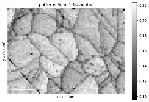
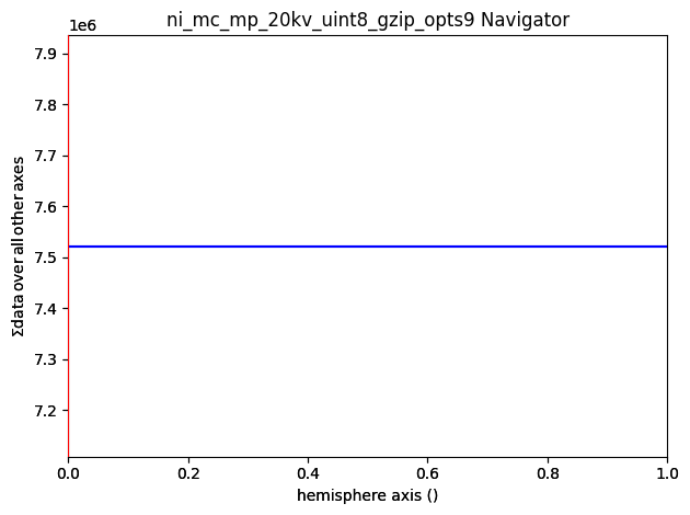
Correlating results from e.g. crystal and phase structure determination, i.e. indexing, with experimental patterns is important when validating the indexing results. When calling plot() without any input parameters, the navigator map is a grey scale image with pixel values corresponding to the sum of all detector intensities within that pattern

s.plot()

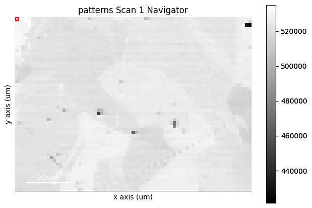
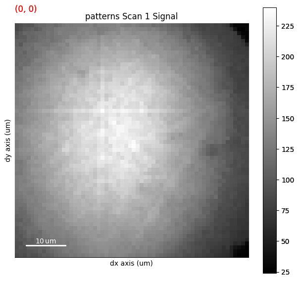
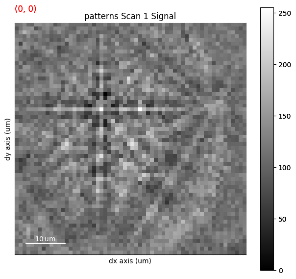
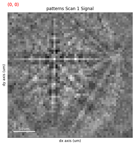
The upper panel shows the navigation axes, in this case 2D. The current navigation position is highlighted in the upper left corner as a red square the size of one pixel. We can change the size of the square with +/-. The square can be moved either by the keyboard arrows or the mouse. The lower panel shows the pattern on the detector in the current navigation position.

Any BaseSignal signal with a 2D signal_shape corresponding to the scan navigation_shape can be passed in to the navgiator parameter in plot(). This includes a virtual image showing diffraction contrast, any quality metric map, or an inverse pole figure (IPF) or phase map.

Virtual image

A virtual backscatter electron (VBSE) image created from any detector region of interest with the get_virtual_bse_intensity() method or get_rgb_image() explained in the virtual backscatter electron imaging tutorial, can be used as a navigator for a scan s

vbse_imager = kp.imaging.VirtualBSEImager(s)
print(vbse_imager)
print(vbse_imager.grid_shape)

VirtualBSEImager for <EBSD, title: patterns Scan 1, dimensions: (75, 55|60, 60)>
(5, 5)

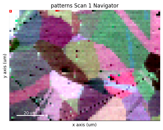
maps_vbse_rgb = vbse_imager.get_rgb_image(r=(3, 1), b=(3, 2), g=(3, 3))
maps_vbse_rgb

<VirtualBSEImage, title: , dimensions: (|75, 55)>

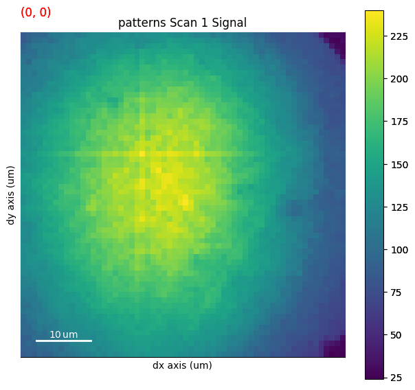
s.plot(navigator=maps_vbse_rgb, cmap="viridis")

Any image

An image made into a Signal2D can be used as navigators. This includes quality metric maps such as the image quality map, calculated using get_image_quality()

s.remove_static_background()
s.remove_dynamic_background()

[########################################] | 100% Completed | 202.60 ms
[########################################] | 100% Completed | 707.52 ms

maps_iq = s.get_image_quality()
s_iq = hs.signals.Signal2D(maps_iq)
s.plot(navigator=s_iq)

[########################################] | 100% Completed | 403.25 ms

We can obtain an RGB signal from an RGB image using get_rgb_navigator(). Let’s load an IPF-Z map representing orientations obtained from dictionary indexing in the pattern matching tutorial

maps_ipfz = plt.imread("../_static/image/visualizing_patterns/ni_large_rgb_z.png")
maps_ipfz = maps_ipfz[..., :3]  # Drop the alpha channel
s_ipfz = kp.draw.get_rgb_navigator(maps_ipfz)

s.plot(navigator=s_ipfz, colorbar=False)

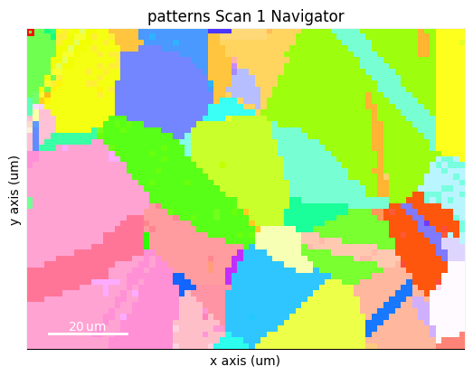
By overlaying the image quality map on the RGB image, we can visualize crystal directions within grains and the grain morphology in the same image

maps_iq_1d = maps_iq.ravel()  # Flat array required by orix
maps_ipfz_1d = maps_ipfz.reshape(-1, 3)
fig = s.xmap.plot(maps_ipfz_1d, overlay=maps_iq_1d, return_figure=True)

By extracting the image array, we can use this map to navigate patterns in

maps_ipfz_iq = fig.axes[0].images[0].get_array()
s_ipfz_iq = kp.draw.get_rgb_navigator(maps_ipfz_iq)
s.plot(s_ipfz_iq)

Plot multiple signals

HyperSpy provides the function plot_signals() to plot multiple signals with the same navigator (detailed in their documentation). Among other uses, this function enables plotting of the experimental and best matching simulated patterns side by side. This can be a powerful visual validation of indexing results. See the pattern matching tutorial for a demonstration.

Plot master patterns

EBSDMasterPattern signals can be navigated along their energy axis and/or their upper/lower hemispheres. Let’s reload the nickel master pattern used in the previous section, but this time in the stereographic projection.

# Only a single energy, 20 keV
mp_stereo = kp.data.nickel_ebsd_master_pattern_small(
    projection="stereographic", hemisphere="both"
)
print(mp_stereo.axes_manager)

<Axes manager, axes: (2|401, 401)>
            Name |   size |  index |  offset |   scale |  units
================ | ====== | ====== | ======= | ======= | ======
      hemisphere |      2 |      0 |       0 |       1 |
---------------- | ------ | ------ | ------- | ------- | ------
           width |    401 |      0 |  -2e+02 |       1 |     px
          height |    401 |      0 |  -2e+02 |       1 |     px

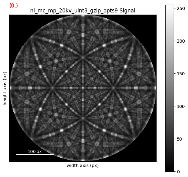
As can be seen from the axes manager, the master pattern has two navigation axes, the upper and lower hemispheres. When plotting, we therefore get a navigation slider

mp_stereo.plot()

We can plot the master pattern on the sphere with EBSDMasterPattern.plot_spherical(). This visualization requires the master pattern to be in the stereographic projection. If the corresponding phase is centrosymmetry, the upper and lower hemispheres are identical, so we only need one of them to cover the sphere. If the phase is non-centrosymmetric, however, both hemispheres must be loaded, as they are unequal. The initial orientation of the sphere corresponds to the orientation of the stereographic and Lambert projections.

mp_stereo.plot_spherical(style="points")

PyVista, required for this plot, is an optional dependency of kikuchipy (see the installation guide for details). Here, the plot uses the static Jupyter backend supported by PyVista. The backend was set in the first notebook cell. When running the notebook locally, we can make the plot interactive setting the backend to "trame". We can pass plotter_kwargs={"notebook": False}" to plot_spherical() if we want to plot the master pattern in a separate window.