
Live notebook
You can run this notebook in a live session ![]() or view it on Github.
or view it on Github.
Multivariate analysis#
See HyperSpy’s user guide for explanations on available multivariate statistical analysis (“machine learning”) methods and more examples of their use.
Denoising EBSD patterns with dimensionality reduction#
Let’s use principal component analysis (PCA) followed by dimensionality reduction to increase the signal-to-noise ratio \(S/N\) in a small Nickel EBSD data set, here called denoising. This denoising is explained further in [Ånes et al., 2020].
[1]:
# Exchange inline for notebook or qt5 (from pyqt) for interactive plotting
%matplotlib inline

import matplotlib.pyplot as plt
import numpy as np

import hyperspy.api as hs
import kikuchipy as kp

s = kp.data.nickel_ebsd_large(allow_download=True)  # External download
s
[1]:
<EBSD, title: patterns Scan 1, dimensions: (75, 55|60, 60)>
Let’s first increase \(S/N\) by removing the undesired static and dynamic backgrounds
[2]:
s.remove_static_background()
s.remove_dynamic_background()
Followed by averaging each pattern with the eight nearest patterns using a Gaussian kernel of \(\sigma = 2\) centered on the pattern being averaged
[3]:
s.average_neighbour_patterns(window="gaussian", std=2)
[########################################] | 100% Completed | 204.84 ms
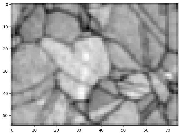
We use the average image quality (IQ) and the IQ map to assess how successful our denoising was. Let’s inspect these before denoising
[4]:
iq1 = s.get_image_quality()
[5]:
print(iq1.mean())

plt.imshow(iq1, cmap="gray")
plt.tight_layout()
0.30131632
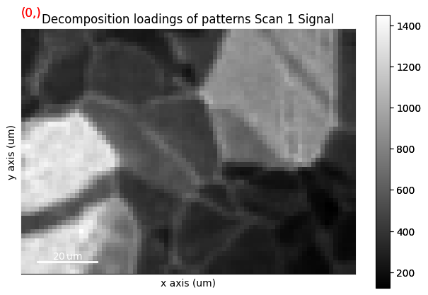
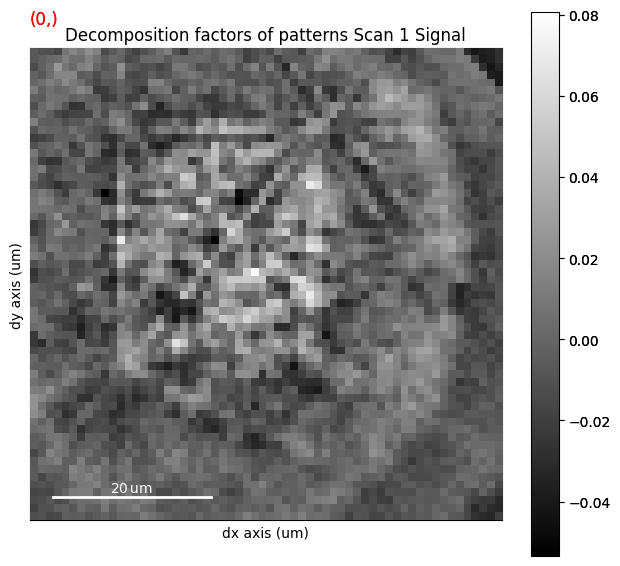
The basic idea of PCA is to decompose the data to a set of values of linearly uncorrelated, orthogonal variables called principal components, or component factors in HyperSpy, while retaining as much as possible of the variation in the data. The factors are ordered by variance. For each component factor, we obtain a component loading, showing the variation of the factor’s strength from one observation point to the next.
Ideally, the first component corresponds to the crystallographic feature most prominent in the data, for example the largest grain, the next corresponds to the second largest feature, and so on, until the later components at some point contain only noise. If this is the case, we can increase \(S/N\) by reconstructing our EBSD signal from the first \(n\) components only, discarding the later components.
PCA decomposition in HyperSpy is done via singular value decomposition (SVD) as implemented in scikit-learn. To prevent number overflow during the decomposition, our detector pixels data type must be of the float or complex type
[6]:
dtype_orig = s.data.dtype
s.change_dtype("float32")
To reduce the effect of the mean intensity per pattern on the overall variance in the entire dataset, we center the patterns by subtracting their mean intensity before decomposing. This is done by passing centre="signal". Considering the expected number of components in our small Nickel data set, let’s keep only 100 of the ranked components
[7]:
n_components = 100
s.decomposition(
    algorithm="SVD",
    output_dimension=n_components,
    centre="signal",
)
Decomposition info:
  normalize_poissonian_noise=False
  algorithm=SVD
  output_dimension=100
  centre=signal
[8]:
s.change_dtype(dtype_orig)
We can inspect our decomposition results by clicking through the ranked component factors and their corresponding loading
[9]:
s.plot_decomposition_results()
WARNING | Hyperspy | Navigation sliders not available. No toolkit registered. Install hyperspy_gui_ipywidgets or hyperspy_gui_traitsui GUI elements. (hyperspy.drawing.mpl_he:191)
[10]:
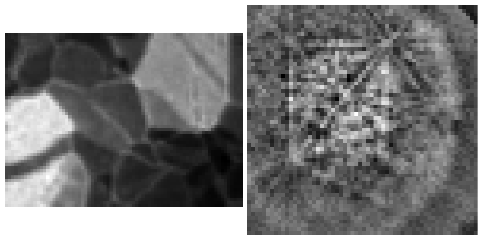
factors = s.learning_results.factors  # (n detector pixels, m components)
sig_shape = s.axes_manager.signal_shape[::-1]
loadings = s.learning_results.loadings  # (n patterns, m components)
nav_shape = s.axes_manager.navigation_shape[::-1]

fig, ax = plt.subplots(ncols=2, figsize=(10, 5))
ax[0].imshow(loadings[:, 0].reshape(nav_shape), cmap="gray")
ax[0].axis("off")
ax[1].imshow(factors[:, 0].reshape(sig_shape), cmap="gray")
ax[1].axis("off")
fig.tight_layout(w_pad=0)
We can also inspect the so-called scree plot of the proportion of variance as a function of the ranked components
[11]:
_ = s.plot_explained_variance_ratio(n=n_components)
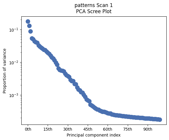
The slope of the proportion of variance seems to fall after about 50-60 components. Let’s inspect the components 60-64 for any useful signal
[12]:
fig, ax = plt.subplots(ncols=4, figsize=(15, 5))
for i in range(4):
    factor_idx = i + 59
    factor = factors[:, factor_idx].reshape(sig_shape)
    factor_iq = kp.pattern.get_image_quality(factor)
    ax[i].imshow(factor, cmap="gray")
    ax[i].set_title(f"#{factor_idx}, IQ = {np.around(factor_iq, 2)}")
    ax[i].axis("off")
fig.tight_layout()
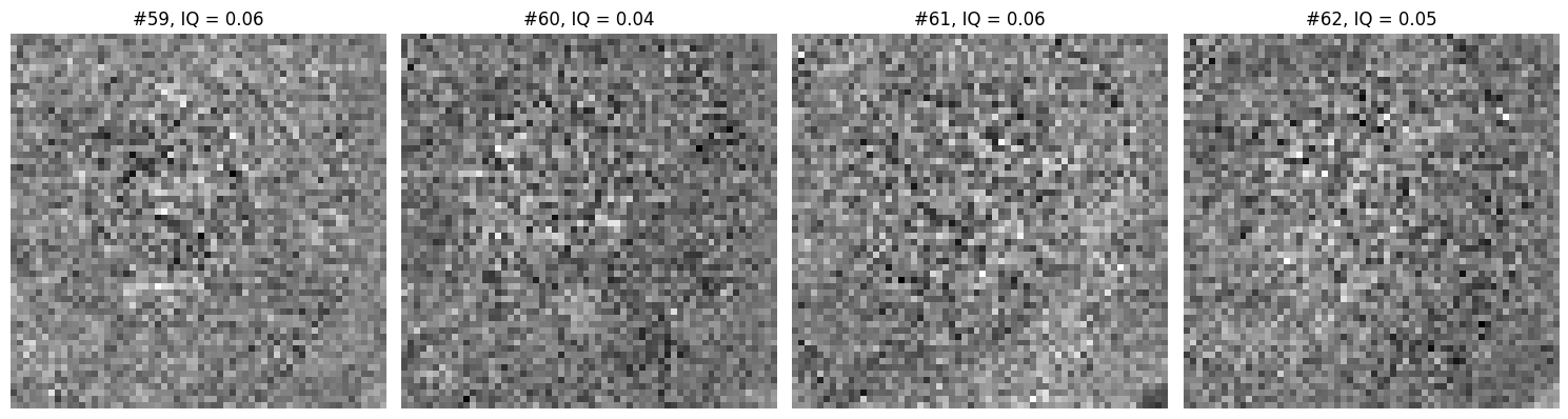
It seems reasonable to discard these components. Note, however, that the selection of a suitable number of components is in general difficult.
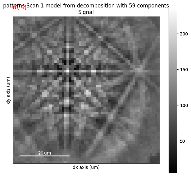
[13]:
s2 = s.get_decomposition_model(components=59)
[14]:
iq2 = s2.get_image_quality()
iq2.mean()
[14]:
np.float32(0.33968797)
[15]:
fig, ax = plt.subplots(ncols=2, figsize=(15, 4))
im0 = ax[0].imshow(iq1, cmap="gray")
ax[0].axis("off")
fig.colorbar(im0, ax=ax[0], pad=0.01, label="IQ before denoising")
im1 = ax[1].imshow(iq2, cmap="gray")
ax[1].axis("off")
fig.colorbar(im1, ax=ax[1], pad=0.01, label="IQ after denoising")
fig.tight_layout(w_pad=-10)
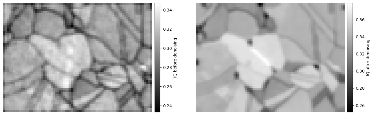
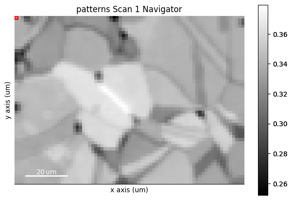
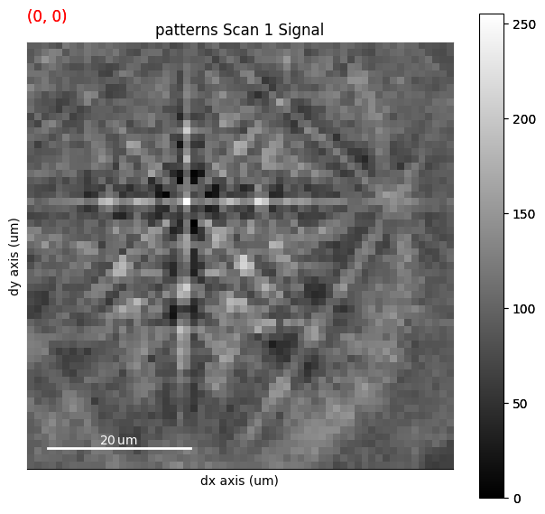
We see that the average IQ increased from 0.30 to 0.34. We can inspect the results per pattern by plotting the signal before and after denoising in the same navigator
[16]:
hs.plot.plot_signals([s, s2], navigator=hs.signals.Signal2D(iq2))