

Live notebook
You can run this notebook in a live session ![]() or view it on Github.
or view it on Github.
Hybrid indexing#
In this tutorial, we combine Hough indexing (HI), dictionary indexing (DI), and refinement in a hybrid indexing approach. HI is generally much faster than DI, but less robust towards noisy patterns. To make good use of both indexing approaches, we can index all patterns with HI, identify badly indexed map points, and re-index these with DI. Before combining orientations obtained from HI and DI into a single map, we must refine them. As always, it is important to validate intermediate results after each step by inspecting quality metrics, geometrical simulations etc.
We demonstrate this workflow with an EBSD dataset from a single-phase recrystallized nickel sample. The dataset is available in a repository on Zenodo at [Ånes et al., 2019]. The dataset is number ten (24 dB) out of a series of ten datasets in the repostiroy, taken with increasing gain (0-24 dB). It is very noisy, so we will average each pattern with its nearest neighbours before indexing.
The complete workflow is:
Load, process, and inspect the full dataset
Calibrate geometry to obtain a plane of projection centers (one for each map point)
Hough indexing of all patterns
Identify (bad) points for re-indexing
Re-indexing with dictionary indexing
Refine Hough indexed and dictionary indexed points
Merge results
Validate results
Let’s start by important the necessary libraries
[1]:
# Exchange inline for notebook or qt5 (from pyqt) for interactive plotting
%matplotlib inline

import matplotlib.pyplot as plt
import numpy as np

from diffsims.crystallography import ReciprocalLatticeVector
import hyperspy.api as hs
import kikuchipy as kp
from orix import plot, sampling
from orix.crystal_map import PhaseList
from orix.vector import Vector3d

plt.rcParams.update(
    {
        "figure.facecolor": "w",
        "font.size": 15,
        "figure.dpi": 75,
    }
)
Load, process and inspect data#
[2]:
s = kp.data.ni_gain(10, allow_download=True)  # ~100 MB into memory
s
Downloading file 'data/scan10_gain24db.zip' from 'https://zenodo.org/record/7498632/files/scan10_gain24db.zip' to '/Users/hakon/Library/Caches/kikuchipy/0.12.0'.
Unzipping contents of '/Users/hakon/Library/Caches/kikuchipy/0.12.0/data/scan10_gain24db.zip' to '/Users/hakon/Library/Caches/kikuchipy/0.12.0/data/ni_gain/10'
[2]:
<EBSD, title: Pattern, dimensions: (200, 149|60, 60)>
Enhance the Kikuchi pattern with background correction
[3]:
s.remove_static_background()
s.remove_dynamic_background()
Average each pattern to its eight nearest neighbors in a Gaussian kernel with a standard deviation of 1
[4]:
window = kp.filters.Window("gaussian", std=1)
s.average_neighbour_patterns(window)
[########################################] | 100% Completed | 318.70 ms
Inspect an image quality map (pattern sharpness, not to be confused with image/pattern quality determined from the height of peaks in the Radon transform)
[5]:
maps_iq = s.get_image_quality()
Inspect patterns in the image quality map
[6]:
# Move the pointer programmatically to the center of a large grain
s.axes_manager.indices = (156, 80)

s.plot(hs.signals.Signal2D(maps_iq))
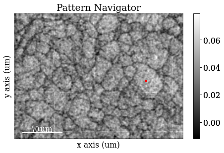
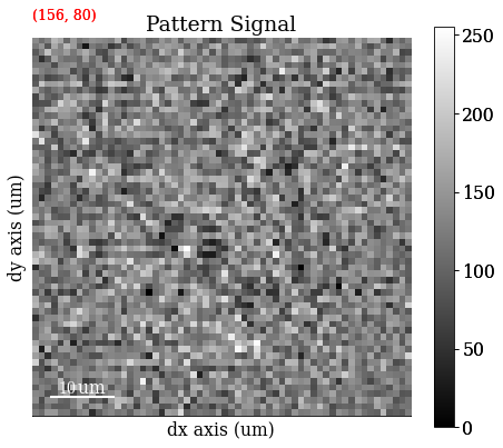
The image quality map is very noisy. However, we might be able to convince ourselves that the darker lines are grain boundaries. The map is noisy because the patterns are noisy. The pattern shown is from the center of a large grain on the right side of the map from the small red square (the pointer). Even though the material is well recrystallized with appreciably large grains, the pattern is very noisy. But again, we might be able to convince ourselves that the pattern shows “correlated noise”, e.g. a couple of zones axes (darker regions in the pattern) and some bands delineated by darker lines on each side of the band.
Calibrate geometry#
Seven calibration patterns of high quality was acquired prior to acquiring the full dataset above. These were acquired to calibrate the sample-detector geometry. The detector was mounted with the screen normal at 0\(^{\circ}\) to the horizontal. The sample was tilted to 70\(^{\circ}\) from the horizontal. We assume these tilts to be correct. What remains is to determine a plane of projection centers (PCs), one for each map point. Since we know the detector pixel size (~70 μm on the NORDIF UF-1100 detector), we can extrapolate this plane of PCs from a mean PC. The workflow is as follows:
Estimate PCs from an initial guess using Hough indexing
Hough indexing of calibration patterns using estimated PCs
Refine Hough indexed orientations and estimated PCs using pattern matching
Extrapolate plane of PCs from mean of refined PCs
We validate the results after each step.
Load calibration patterns
[7]:
[7]:
<EBSD, title: Calibration patterns, dimensions: (7|480, 480)>
Remove static and dynamic background
Note
Trial-and-error showed that the dataset of patterns previously loaded, s, were better indexed after subtracting the static and dynamic background rather than dividing by them (the image/pattern quality maps also show a more meaningful contrast). No clear difference in indexing results are observed for the calibration patterns. See the tutorial on pattern processing for more details.
[8]:
s_cal.remove_static_background("divide")
s_cal.remove_dynamic_background("divide")
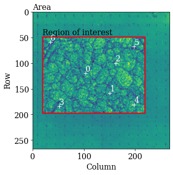
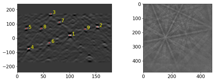
Extract the positions of the calibration patterns (possibly outside the region of interest [ROI]) and the shape and position of the ROI relative to the area imaged in an overview secondary electron image. This information is read with the calibration patterns from the NORDIF settings file.
[9]:
omd = s_cal.original_metadata
Plot calibration pattern map locations
[10]:
kp.draw.plot_pattern_positions_in_map(
    rc=omd.calibration_patterns.indices_scaled,
    roi_shape=omd.roi.shape_scaled,
    roi_origin=omd.roi.origin_scaled,
    roi_image=maps_iq,
    area_shape=omd.area.shape_scaled,
    area_image=omd.area_image,
    color="w",
)
Hough indexing requires a phase list in order to make a look-up table of interplanar angles to compare the detected angles to (from combinations of bands). See the Hough indexing tutorial for more details. Since we later on need a dynamically simulated master pattern of nickel (simulated with EMsoft), we will load this here and use the phase description of the master pattern in the phase list.
Note
PyEBSDIndex is an optional dependency of kikuchipy, and can be installed with both pip and conda (from conda-forge). To install PyEBSDIndex, see their installation instructions.
[11]:
# kikuchipy.data.nickel_ebsd_master_pattern_small() is a lower-resolution alternative
mp = kp.data.ebsd_master_pattern(
    "ni", projection="lambert", energy=20, allow_download=True
)
mp
[11]:
<EBSDMasterPattern, title: ni_mc_mp_20kv, dimensions: (|1001, 1001)>
[12]:
phase = mp.phase
phase
[12]:
<name: ni. space group: Fm-3m. point group: m-3m. proper point group: 432. color: tab:blue>
Create a PyEBSDIndex indexer to use with Hough indexing. We should pass our own reflector list to the indexer, so we generate a set of high-symmetry reflectors \(\mathbf{g}\) (see the tutorial on geometrical simulations for details)
[13]:
g = ReciprocalLatticeVector.from_min_dspacing(phase.deepcopy(), 0.07)
g.sanitise_phase()  # "Fill atoms in unit cell", required for structure factor
g.calculate_structure_factor()
F = abs(g.structure_factor)
g = g[F > 0.12 * F.max()]
g.print_table()
 h k l      d     |F|_hkl   |F|^2   |F|^2_rel   Mult
 1 1 1    0.203     0.4      0.2      100.0      8
 2 0 0    0.176     0.3      0.1       60.9      6
 2 2 0    0.125     0.1      0.0       8.7       12
 3 1 1    0.106     0.1      0.0       2.0       24
We get the indexer from the detector attached to the calibration pattern signal
[14]:
det_cal = s_cal.detector
phase_list = PhaseList(phase)
indexer = det_cal.get_indexer(phase_list, g.unique(True))
Estimate PCs from an initial guess (based on previous experiments) and print the mean and standard deviation
[15]:
[0.41795065 0.22155998 0.504981  ]
[0.0054912  0.00651565 0.00551478]
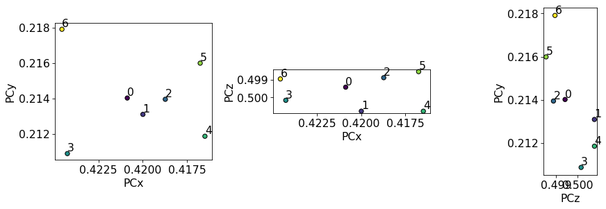
Compare the distribution of PCs to the above plotted map locations (especially PCx vs. PCy)
[16]:
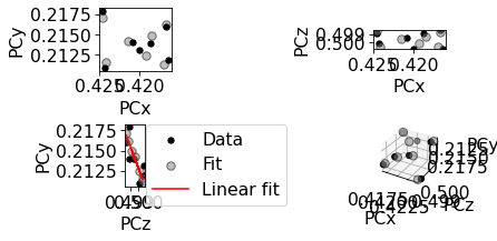
det_cal.plot_pc("scatter", annotate=True)
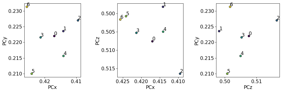
We see no direct correlation between the sample positions and the PCs. Let’s index the calibration patterns using these PCs and compare the solutions’ band positions to the actual bands. We update our indexer instance with the estimated PCs.
[17]:
indexer.PC = det_cal.pc
xmap_cal = s_cal.hough_indexing(
    phase_list=phase_list, indexer=indexer, verbose=2
)
Hough indexing with PyEBSDIndex information:
  PyOpenCL: True
  Projection center (Bruker, mean): (0.418, 0.2216, 0.505)
  Indexing 7 pattern(s) in 1 chunk(s)
Radon Time: 0.005836875003296882
Convolution Time: 0.02429116700659506
Peak ID Time: 0.00881512499472592
Band Label Time: 0.012671916992985643
Total Band Find Time: 0.05173937500512693
Band Vote Time:  0.0036097909905947745
  Indexing speed: 104.87820 patterns/s
Check indexed orientations by plotting geometrical simulations on top of the patterns
[18]:
simulator = kp.simulations.KikuchiPatternSimulator(g)
sim_cal = simulator.on_detector(det_cal, xmap_cal.rotations)
Finding bands that are in some pattern:
[########################################] | 100% Completed | 105.65 ms
Finding zone axes that are in some pattern:
[########################################] | 100% Completed | 105.77 ms
Calculating detector coordinates for bands and zone axes:
[########################################] | 100% Completed | 106.81 ms
[19]:
# Enhance meaningful contrast for visualization
s_cal2 = s_cal.normalize_intensity(dtype_out="float32", inplace=False)
fig, axes = plt.subplots(ncols=3, nrows=3, figsize=(12, 12))
axes = axes.ravel()
for i in range(xmap_cal.size):
axes[i].imshow(s_cal2.inav[i].data, cmap="gray", vmin=-3, vmax=3)
lines = sim_cal.as_collections(i, lines_kwargs={"color": "w"})[0]
axes[i].add_collection(lines)
axes[i].text(5, 10, i, c="w", va="top", ha="left")
_ = [ax.axis("off") for ax in axes]
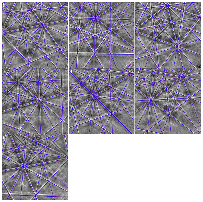
fig.subplots_adjust(wspace=0.01, hspace=0.01)
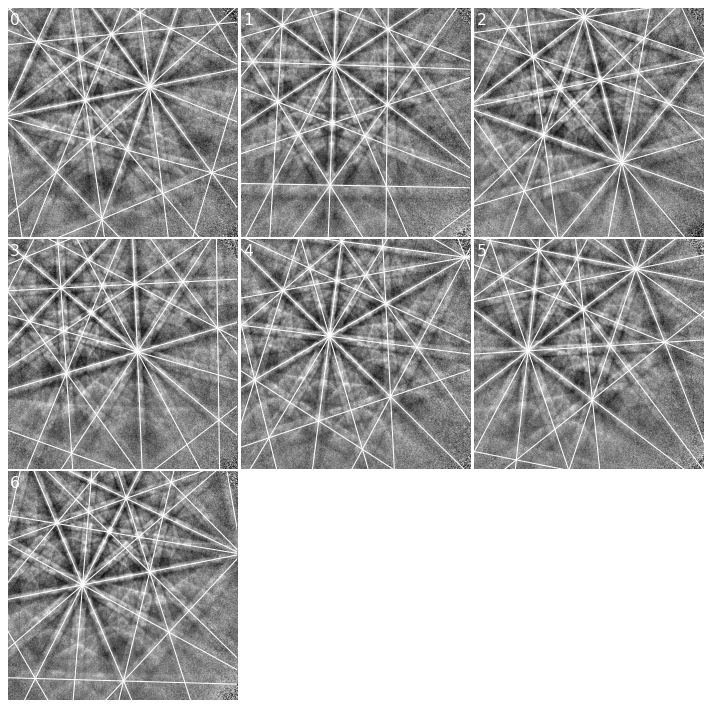
Most lines align quite well with the bands. Some of them, especially in the lower part of the patterns and on wide bands, do not follow the band center, though (see e.g. pattern 4). Let’s refine these solutions using dynamical simulations
[20]:
xmap_cal_ref, det_cal_ref = s_cal.refine_orientation_projection_center(
    xmap=xmap_cal,
    detector=det_cal,
    master_pattern=mp,
    energy=20,
    method="LN_NELDERMEAD",
    trust_region=[5, 5, 5, 0.05, 0.05, 0.05],  # Sufficiently wide
    rtol=1e-5,
    # One pattern per iteration to utilize all CPUs
    chunk_kwargs=dict(chunk_shape=1),
)
Refinement information:
  Method: LN_NELDERMEAD (local) from NLopt
  Trust region (+/-): [5.   5.   5.   0.05 0.05 0.05]
  Relative tolerance: 1e-05
Refining 7 orientation(s) and projection center(s):
[########################################] | 100% Completed | 7.43 sms
Refinement speed: 0.94202 patterns/s
Check quality metrics
0.46331794347081867
291.14285714285717
Check deviations from Hough indexed solutions (it is important that these deviations are within our trust region above)
[22]:
[1.34451885 1.47180963 2.21946645 1.38628363 0.82136501 0.87480888
 1.57285028]
[0.00924619 0.01338432 0.01753987]
Get geometrical simulations from refined orientations and PCs and add lines from these simulations (in red) to the existing figure
[23]:
sim_cal_ref = simulator.on_detector(det_cal_ref, xmap_cal_ref.rotations)
Finding bands that are in some pattern:
[########################################] | 100% Completed | 105.58 ms
Finding zone axes that are in some pattern:
[########################################] | 100% Completed | 105.86 ms
Calculating detector coordinates for bands and zone axes:
[########################################] | 100% Completed | 106.93 ms
[24]:
for i in range(xmap_cal_ref.size):
    lines = sim_cal_ref.as_collections(i)[0]
    axes[i].add_collection(lines)
fig
[24]:
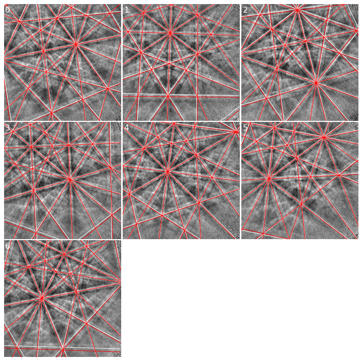
We see that the red lines align better with wider bands and bands in the lower part of the patterns (where the deviations are greater).
Check the refined PCs
[25]:
det_cal_ref.plot_pc("scatter", annotate=True)
We now see that the patterns align quite well compared to the sample positions. We will therefore attempt to fit a plane to these PCs using an affine transformation (see the tutorial on PC plane fitting for more details). Note that if the PCs hadn’t aligned as nicely as here, we should instead extrapolate a plane of PCs from an average; this procedure is detailed in another tutorial.
[26]:
pc_indices = omd.calibration_patterns.indices_scaled.copy()
pc_indices -= omd.roi.origin_scaled
pc_indices = pc_indices.T

det_cal_fit = det_cal_ref.fit_pc(
    pc_indices,
    map_indices=np.indices(s.axes_manager.navigation_shape[::-1]),
    transformation="affine",
)
print(det_cal_fit.pc_average)

# Sample tilt
print(det_cal_fit.sample_tilt)

# Max. deviation between experimental and fitted PC
pc_diff_fit = det_cal_ref.pc - det_cal_fit.pc[tuple(pc_indices)]
print(abs(pc_diff_fit.reshape(-1, 3)).mean(axis=0))
[0.42070818 0.21404481 0.49961799]
69.76546616579716
[0.0003229  0.0005966  0.00033309]
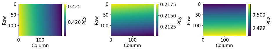
Check the plane of PCs
[27]:
det_cal_fit.plot_pc()
As a final validation of this plane of PCs, we will refine the (refined) orientations using a fixed PC for each pattern, taken from the plane of PCs
[28]:
det_cal_fit2 = det_cal_fit.deepcopy()
det_cal_fit2.pc = det_cal_fit2.pc[tuple(pc_indices)]
[29]:
Refinement information:
  Method: LN_NELDERMEAD (local) from NLopt
  Trust region (+/-): [10 10 10]
  Relative tolerance: 1e-05
Refining 7 orientation(s):
[########################################] | 100% Completed | 1.25 sms
Refinement speed: 5.57746 patterns/s
0.4632044647421156
74.57142857142857
[31]:
angles_cal2 = xmap_cal_ref.orientations.angle_with(
    xmap_cal_ref2.orientations, degrees=True
)
print(angles_cal2)
[0.22046472 0.32424457 0.14197507 0.15490383 0.29473138 0.20720924
 0.31697432]
Get geometrical simulations and add a third set of lines (in blue) to the existing figure
[32]:
sim_cal_ref2 = simulator.on_detector(det_cal_fit2, xmap_cal_ref2.rotations)
Finding bands that are in some pattern:
[########################################] | 100% Completed | 105.83 ms
Finding zone axes that are in some pattern:
[########################################] | 100% Completed | 106.17 ms
Calculating detector coordinates for bands and zone axes:
[########################################] | 100% Completed | 107.30 ms
[33]:
[33]:
Hough indexing of all patterns#
Now that we are confident of our geometry calibration, we can index all patterns in our noisy experimental dataset.
Copy the detector with the calibrated PCs and update the detector shape to match our experimental patterns
[34]:
det = det_cal_fit.deepcopy()
det.shape = s.detector.shape
det
[34]:
EBSDDetector
  shape (Ny, Nx):     (60, 60)
  pc (PCx, PCy, PCz): (0.421, 0.214, 0.5)
  sample_tilt:        69.765°
  tilt:               0.0°
  azimuthal:          0.0°
  twist:              0.0°
  binning:            1
  px_size:            1.0 um
Get a new indexer
[35]:
indexer = det.get_indexer(phase_list, g.unique(True), rSigma=2, tSigma=2)
Perform Hough indexing with PyEBSDIndex (using the GPU via PyOpenCL, but only a single CPU)
[36]:
xmap_hi = s.hough_indexing(phase_list=phase_list, indexer=indexer, verbose=2)
Hough indexing with PyEBSDIndex information:
  PyOpenCL: True
  Projection center (Bruker, mean): (0.4207, 0.214, 0.4996)
  Indexing 29800 pattern(s) in 57 chunk(s)
Radon Time: 0.2926339150290005
Convolution Time: 2.0258173329784768
Peak ID Time: 0.7259590040921466
Band Label Time: 0.5914002920035273
Total Band Find Time: 3.6442706660018303
Band Vote Time:  0.547384499994223
  Indexing speed: 7041.48457 patterns/s
Our use of PyEBSDIndex here (with PyOpenCL installed) index about 4 000 patterns/s.
Note
Note that PyEBSDIndex can index a lot faster than this by using more CPUs and by passing a file directly (not via NumPy or Dask arrays, as done here) to its indexing functions. See its documentation for details: https://pyebsdindex.readthedocs.io/en/latest.
[37]:
xmap_hi
[37]:
Phase    Orientations         Name  Space group  Point group  Proper point group     Color
   -1     1127 (3.8%)  not_indexed         None         None                None     white
    0   28673 (96.2%)           ni        Fm-3m         m-3m                 432  tab:blue
Properties: fit, cm, pq, nmatch
Scan unit: um
[38]:
# Save HI map
# from orix import io
# io.save("xmap_hi.ang", xmap_hi)
# io.save("xmap_hi.h5", xmap_hi)
PyEBSDIndex could not index some 4% of patterns (too high pattern fit). Let’s check the quality metrics (pattern fit, confidence metric, pattern quality, and the number of detected bands that were assigned an index [“indexed”])
[39]:
aspect_ratio = xmap_hi.shape[1] / xmap_hi.shape[0]
figsize = (8 * aspect_ratio, 4.5 * aspect_ratio)

fig, axes = plt.subplots(nrows=2, ncols=2, figsize=figsize, layout="tight")
for ax, to_plot in zip(axes.ravel(), ["pq", "cm", "fit", "nmatch"]):
    if to_plot == "fit":
        im = ax.imshow(xmap_hi.get_map_data(to_plot), vmin=0, vmax=2)
    else:
        im = ax.imshow(xmap_hi.get_map_data(to_plot))
    fig.colorbar(im, ax=ax, label=to_plot, pad=0.02)
    ax.axis("off")
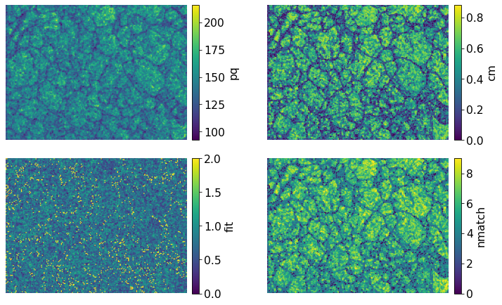
The bright points in the lower left pattern fit map are the points considered not indexed. The confidence metric and number of successfully labeled bands (out of nine) seem to be highest within grains and lowest at grain boundaries. Let’s inspect the spatial variation of “successfully” indexed orientations in an inverse pole figure map (IPF-X)
[40]:
pg = xmap_hi.phases[0].point_group
ckey = plot.IPFColorKeyTSL(pg, Vector3d([1, 0, 0]))
ckey
[40]:
IPFColorKeyTSL, symmetry: m-3m, direction: [1 0 0]
[41]:
rgb_hi = ckey.orientation2color(xmap_hi["indexed"].rotations)
fig = xmap_hi["indexed"].plot(
    rgb_hi, remove_padding=True, return_figure=True
)

# Place color key in bottom right corner, coordinates are
# [left, bottom, width, height]
ax_ckey = fig.add_axes([0.76, 0.08, 0.2, 0.2], projection="ipf", symmetry=pg)
ax_ckey.plot_ipf_color_key(show_title=False)
ax_ckey.patch.set_facecolor("None")
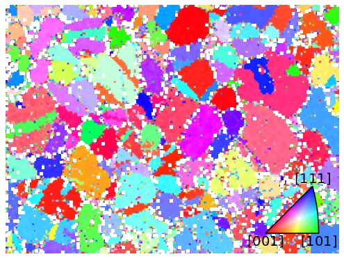
Many points seen as single color deviations from otherwise smooth colors within recrystallized grains are located mostly at grain boundaries.
Identify points for re-indexing#
Let’s see if we can easily separate the good from bad points using any of the quality metrics
[42]:
fig, axes = plt.subplots(ncols=4, figsize=(10, 3), layout="tight")
for ax, to_plot in zip(axes.ravel(), ["pq", "cm", "fit", "nmatch"]):
    _ = ax.hist(xmap_hi["indexed"].prop[to_plot], bins=100)
    ax.set(xlabel=to_plot, ylabel="Frequency")
    if to_plot == "pq":
        ax.ticklabel_format(axis="x", style="sci", scilimits=(0, 0))
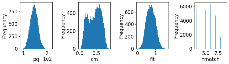
… hm, there is no clear bimodal distribution in any of the histograms except perhaps the pattern misfit. In such cases, one solution is to find the “good” and “bad” points by trial-and-error until a desired separation is achieved. Here, we have combined metrics by trial-and-error to get a plausible separation. Note that other combinations might be better for other datasets.
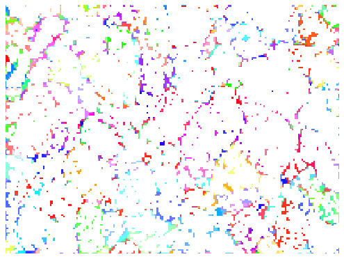
[43]:
mask_reindex = np.logical_or.reduce(
    (
        ~xmap_hi.is_indexed,
        xmap_hi.fit > 0.95,
        xmap_hi.nmatch < 4,
        xmap_hi.cm < 0.25,
    )
)
frac_reindex = mask_reindex.sum() / mask_reindex.size
print(f"Fraction to re-index: {100 * frac_reindex:.2f}%")

# Get colors for all points, even the ones considered not-indexed
rgb_hi_all = ckey.orientation2color(xmap_hi.rotations)

# Get separate arrays for points to keep and to re-index, with in the other
# array as black
rgb_hi_reindex = np.zeros((xmap_hi.size, 3))
rgb_hi_keep = np.zeros_like(rgb_hi_reindex)
rgb_hi_reindex[mask_reindex] = rgb_hi_all[mask_reindex]
rgb_hi_keep[~mask_reindex] = rgb_hi_all[~mask_reindex]

nav_shape = xmap_hi.shape + (3,)

fig, (ax0, ax1) = plt.subplots(ncols=2, figsize=(12, 5), layout="tight")
ax0.imshow(rgb_hi_keep.reshape(nav_shape))
ax1.imshow(rgb_hi_reindex.reshape(nav_shape))
for ax, title in zip([ax0, ax1], ["Keep", "Re-index with DI"]):
    ax.axis("off")
    ax.set(title=title)
Fraction to re-index: 43.87%

There are some spurious points still left among the points to keep. Otherwise, the inverse pole figure map looks fairly convincing.
Make a 2D navigation mask where points to re-index are set to False.
Re-indexing with dictionary indexing#
To generate the dictionary of nickel patterns, we need to sample orientation space at a sufficiently high resolution (here 2\(^{\circ}\)) with a fixed calibration geometry (PC). See the pattern matching tutorial for details.
[45]:
R = sampling.get_sample_fundamental(resolution=2, point_group=pg)
R
[45]:
Rotation (100347,)
[[ 0.8541 -0.3536 -0.3536 -0.1435]
 [ 0.8541 -0.3536 -0.3536  0.1435]
 [ 0.8541 -0.3536 -0.1435 -0.3536]
 ...
 [ 0.8541  0.3536  0.1435  0.3536]
 [ 0.8541  0.3536  0.3536 -0.1435]
 [ 0.8541  0.3536  0.3536  0.1435]]
[46]:
det_pc1 = det.deepcopy()
det_pc1.pc = det_pc1.pc_average

det_pc1.pc
[46]:
array([[0.42070818, 0.21404481, 0.49961799]])
[47]:
sim = mp.get_patterns(
    rotations=R,
    detector=det_pc1,
    energy=20,
    chunk_shape=R.size // 20,
)
sim
[47]:
|
|
We only match the intensities within a circular mask (note the inversion!)
[48]:
signal_mask = kp.filters.Window("circular", det.shape).astype(bool)
signal_mask = ~signal_mask
Perform dictionary indexing of the patterns and intensities marked as False in the navigation and signal masks
[49]:
xmap_di = s.dictionary_indexing(
    sim,
    keep_n=1,
    navigation_mask=nav_mask,
    signal_mask=signal_mask,
)
Dictionary indexing information:
  Phase name: ni
  Matching 13072/29800 experimental pattern(s) to 100347 dictionary pattern(s)
  NormalizedCrossCorrelationMetric: float32, greater is better, rechunk: False, navigation mask: True, signal mask: True
100%|████████████████████████████████████████████████████████████████████████████████████████████████████████████████████████████████████████████████████████████████████████████████| 21/21 [00:27<00:00, 1.33s/it]
Indexing speed: 469.09164 patterns/s, 47071938.93988 comparisons/s
[50]:
# Save DI map
# io.save("xmap_di.h5", xmap_di)
We see that HI is > 10x faster than DI.
[51]:
xmap_di.scores.mean()
[51]:
np.float32(0.16086558)
An average correlation score of about 0.15 is low but OK, since we can refine the solutions and would expect a higher score from this. The IPF-Z map looks plausible, though, which it did not from these patterns after HI.
Refine Hough indexed and dictionary indexed points#
First we specify common refinement parameters, so that the scores obtain can be compared. This is very important!
[53]:
ref_kw = {
    "detector": det,
    "master_pattern": mp,
    "energy": 20,
    "signal_mask": signal_mask,
    "method": "LN_NELDERMEAD",
    "trust_region": [5, 5, 5],
}
Of the Hough indexed solutions, we only want to refine those that are not re-indexed using dictionary indexing. We therefore pass the navigation mask, but have to take care to set those points that we want to index to False
[54]:
xmap_hi_ref = s.refine_orientation(
    xmap_hi, navigation_mask=~nav_mask, **ref_kw
)
Refinement information:
  Method: LN_NELDERMEAD (local) from NLopt
  Trust region (+/-): [5 5 5]
  Relative tolerance: 0.0001
Refining 16728 orientation(s):
[########################################] | 100% Completed | 25.24 ss
Refinement speed: 661.57123 patterns/s
0.2428839271225054
155
An average correlation score of about 0.24 is OK.
We now refine the re-indexed points. No navigation mask is necessary, since the crystal map returned from DI has a mask keeping track of which points are “in the data” via CrystalMap.is_in_data.
[56]:
xmap_di_ref = s.refine_orientation(xmap_di, **ref_kw)
Refinement information:
  Method: LN_NELDERMEAD (local) from NLopt
  Trust region (+/-): [5 5 5]
  Relative tolerance: 0.0001
Refining 13072 orientation(s):
[########################################] | 100% Completed | 20.18 ss
Refinement speed: 646.79388 patterns/s
0.2045177728755028
167
An average correlation score of about 0.20 is still OK.
Merge results#
We can now merge the results, taking care to pass the navigation mask where each refined map should be considered. Since only the points not in the refined HI map were indexed with DI, the same mask can be used in both cases.
[58]:
xmap_ref = kp.indexing.merge_crystal_maps(
    [xmap_hi_ref, xmap_di_ref], navigation_masks=[~nav_mask, nav_mask]
)
[59]:
[59]:
Phase    Orientations  Name  Space group  Point group  Proper point group     Color
    0  29800 (100.0%)    ni        Fm-3m         m-3m                 432  tab:blue
Properties: scores, merged_scores
Scan unit: um
We see that we have a complete map for all our points!
[60]:
# Save final refined combined map
# io.save("xmap_ref.ang", xmap_ref)
# io.save("xmap_ref.h5", xmap_ref)
Validate indexing results#
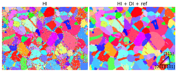
Finally, we can compare the IPF-X maps with HI only and after re-indexing, refinement and combination
[61]:
rgb_ref = ckey.orientation2color(xmap_ref.orientations)
rgb_shape = xmap_ref.shape + (3,)

fig, (ax0, ax1) = plt.subplots(ncols=2, figsize=(12, 5))
ax0.imshow(rgb_hi_all.reshape(rgb_shape))
ax1.imshow(rgb_ref.reshape(rgb_shape))
for ax, title in zip([ax0, ax1], ["HI", "HI + DI + ref"]):
    ax.axis("off")
    ax.set(title=title)

ax_ckey = fig.add_axes(
    [0.805, 0.21, 0.1, 0.1], projection="ipf", symmetry=pg
)
ax_ckey.plot_ipf_color_key(show_title=False)
ax_ckey.patch.set_facecolor("None")
_ = [t.set_fontsize(15) for t in ax_ckey.texts]

fig.subplots_adjust(wspace=0.02)
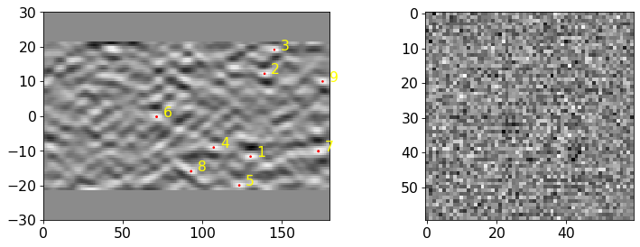
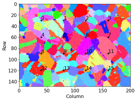
We extract a grid of patterns and plot the geometrical simulations on top of these patterns
[62]:
s.xmap = xmap_ref
s.detector = det
[63]:
grid_shape = (4, 4)
s_grid, idx = s.extract_grid(grid_shape, return_indices=True)
[64]:
kp.draw.plot_pattern_positions_in_map(
    rc=idx.reshape((2, -1)).T,
    roi_shape=xmap_ref.shape,
    roi_image=rgb_ref.reshape(rgb_shape),
)
[65]:
sim_grid = simulator.on_detector(
    s_grid.detector, s_grid.xmap.rotations.reshape(*grid_shape)
)
Finding bands that are in some pattern:
[########################################] | 100% Completed | 100.85 ms
Finding zone axes that are in some pattern:
[########################################] | 100% Completed | 105.90 ms
Calculating detector coordinates for bands and zone axes:
[########################################] | 100% Completed | 106.84 ms
[66]:
fig, axes = plt.subplots(
    nrows=grid_shape[0], ncols=grid_shape[1], figsize=(12, 12)
)
for idx in np.ndindex(grid_shape):
    ax = axes[idx]
    ax.imshow(s_grid.data[idx] * ~signal_mask, cmap="gray")
    lines = sim_grid.as_collections(idx, lines_kwargs=dict(color="k"))[0]
    ax.add_collection(lines)
    ax.axis("off")
    ax.text(
        0,
        1,
        np.ravel_multi_index(idx, grid_shape),
        va="top",
        ha="left",
        c="w",
    )
fig.subplots_adjust(wspace=0.02, hspace=0.02)
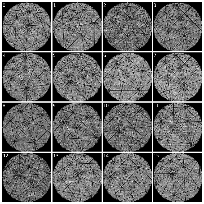
It’s difficult to see any bands in these very noisy patterns… There at least seems to be a correlation between darker regions in the patterns (not the corners) and zone axes, which is expected.
In conclusion, by combining the speed of Hough indexing with the robustness towards noise of dictionary indexing, a dataset can be indexed in a shorter time and achieve about the same results as with DI (and refinement) only.
What’s next?#
Can we improve indexing results by improving further the signal-to-noise ratio in our very noisy EBSD patterns? Instead of the “naive” Gaussian kernel used in neighbour pattern averaging, we could try out a more sophisticated kernel with non-local pattern averaging (NLPAR) from PyEBSDIndex. More details are found in their NLPAR tutorial.