
plot_pc#
- EBSDDetector.plot_pc(mode: Literal['map', 'scatter', '3d'] = 'map', return_figure: Literal[False] = False, orientation: Literal['horizontal', 'vertical'] = 'horizontal', annotate: bool = False, figure_kwargs: dict | None = None, **kwargs) None[source]#
- EBSDDetector.plot_pc(mode: Literal['map', 'scatter', '3d'] = 'map', return_figure: Literal[True] = True, orientation: Literal['horizontal', 'vertical'] = 'horizontal', annotate: bool = False, figure_kwargs: dict | None = None, **kwargs) mfigure.Figure
Plot all projection centers (PCs).
- Parameters:
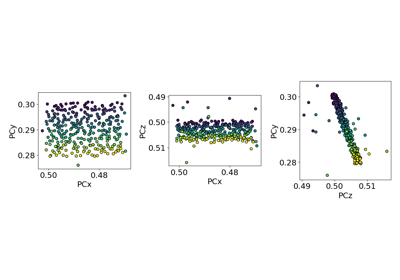
- mode
String describing how to plot PCs. Options are “map” (default), “scatter” and “3d”. If map mode,
navigation_dimensionmust be 2.- return_figure
Whether to return the figure (default is False).
- orientation
Whether to align the plots in a “horizontal” (default) or “vertical” orientation.
- annotate
Whether to label each pattern with its 1D index into
pc_flattenedwhen mode is “scatter”. Default is False.- figure_kwargs
Keyword arguments to pass to
matplotlib.pyplot.figure()upon figure creation. Note thatlayout="tight"is used by default unless another layout is given.- **kwargs
Keyword arguments passed to the plotting function, which is
imshow()if mode is “map”,scatter()if mode is “scatter”, andscatter()if mode is “3d”.
- Returns:
figFigure is returned if return_figure is True.