Plot projection center on the detector

This example shows how to plot the projection/pattern center (PC) on an EBSDDetector. See the detector class documentation for further details on the definition of the PC and gnomonic coordinates.

Imports.

import matplotlib.pyplot as plt

import kikuchipy as kp

Create an EBSD detector with a binning of 8 and a single projection/pattern (PC) center given in EDAX’ definition, \((x^{*}, y^{*}, z^{*}) = (0.421, 0.779, 0.505)\).

det = kp.detectors.EBSDDetector(
    shape=(60, 60),
    pc=[0.421, 0.779, 0.505],
    convention="edax",
    px_size=70,  # Microns
    tilt=5,  # Degrees
    sample_tilt=70,  # Degrees
    binning=8,
)
print(det)

EBSDDetector
  shape (Ny, Nx):     (60, 60)
  pc (PCx, PCy, PCz): (0.421, 0.221, 0.505)
  sample_tilt:        70.0°
  tilt:               5.0°
  azimuthal:          0.0°
  twist:              0.0°
  binning:            8
  px_size:            70.0 um

Load a small test dataset with (60, 60) patterns to plot the PC over.

s = kp.data.nickel_ebsd_small()
print(s)

<EBSD, title: patterns Scan 1, dimensions: (3, 3|60, 60)>

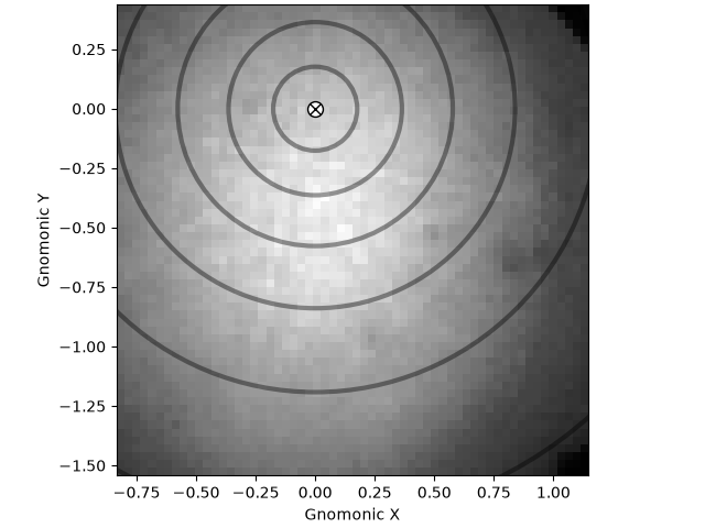
Plot the PC on top of the pattern. Instead of pixels, we show the detector extent in gnomonic coordinates along the x and y axes. We also draw gnomonic circles at an interval of \(10^{\circ}\).

det.plot(
    pattern=s.inav[0, 0].data,
    coordinates="gnomonic",
    draw_gnomonic_circles=True,
)

plt.show()