Live notebook

You can run this notebook in a live session or view it on Github.

Virtual backscatter electron imaging

In this tutorial, we will perform virtual imaging on the EBSD detector to generate maps, known as virtual backscatter electron (VBSE) imaging.

This is useful for getting a qualitative overview of the sample and pattern quality prior to indexing, and can also be useful when interpreting indexing resuls, as they are indexing independent.

Interactive plotting

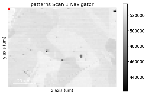
Angle resolved backscatter electron (BSE) imaging can be performed interactively with the method plot_virtual_bse_intensity(), adopted from pyxem, by integrating the intensities within a part, e.g. a (10 x 10) pixel rectangular region of interest (ROI), of the stack of EBSD patterns. Let’s first import necessary libraries and a 13 MB Nickel EBSD data set

# Exchange inline for notebook or qt5 (from pyqt) for interactive plotting
%matplotlib inline

from pathlib import Path
import tempfile

import matplotlib.pyplot as plt
import numpy as np

import hyperspy.api as hs
import kikuchipy as kp


plt.rcParams["font.size"] = 12


s = kp.data.nickel_ebsd_large(allow_download=True)  # External download
s

<EBSD, title: patterns Scan 1, dimensions: (75, 55|60, 60)>

We create a rectangular ROI by specifying the upper left and lower right coordinates of the rectangle in units of the detector pixel size (scale of dx and dy in the signal axes manager)

roi = hs.roi.RectangularROI(left=0, top=0, right=10, bottom=10)
s.plot_virtual_bse_intensity(roi)

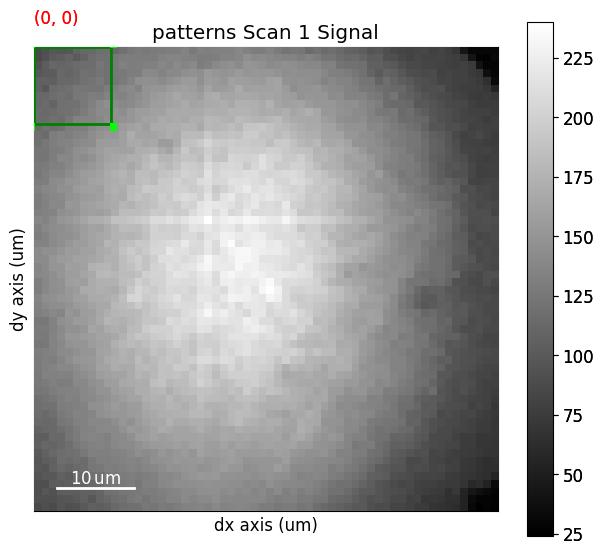
Note that the position of the ROI on the detector is updated during interactive plotting if it is moved around by hand. See HyperSpy’s ROI user guide for more detailed use of ROIs.

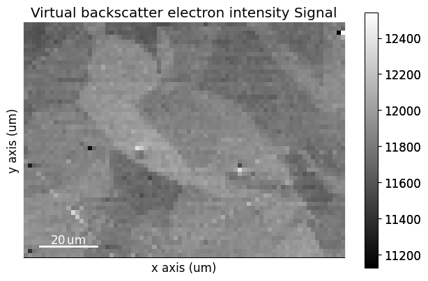
The virtual image, created from integrating the intensities within the ROI, can then be written to an image file using get_virtual_bse_intensity()

vbse = s.get_virtual_bse_intensity(roi)
vbse

<VirtualBSEImage, title: Virtual backscatter electron image, dimensions: (|75, 55)>

temp_dir = Path(tempfile.mkdtemp())
plt.imsave(temp_dir / "vbse1.png", arr=vbse.data)

A VirtualBSEImage instance is returned.

Generate many virtual images

Sometimes we want to get many images from parts of the detector, e.g. like what is demonstrated in the xcdskd project with the angle resolved virtual backscatter electron array (arbse/vbse array). Instead of keeping track of multiple hyperspy.roi.BaseInteractiveROI objects, we can create a detector grid of a certain shape, e.g. (5, 5), and obtain gray scale images, or combine multiple grid tiles in red, green and channels to obtain RGB images.

First, we initialize a virtual BSE image generator, kikuchipy.imaging.VirtualBSEImager, with an EBSD signal, in case the raw EBSD patterns without any background correction or other processing

vbse_imager = kp.imaging.VirtualBSEImager(s)
vbse_imager

VirtualBSEImager for <EBSD, title: patterns Scan 1, dimensions: (75, 55|60, 60)>

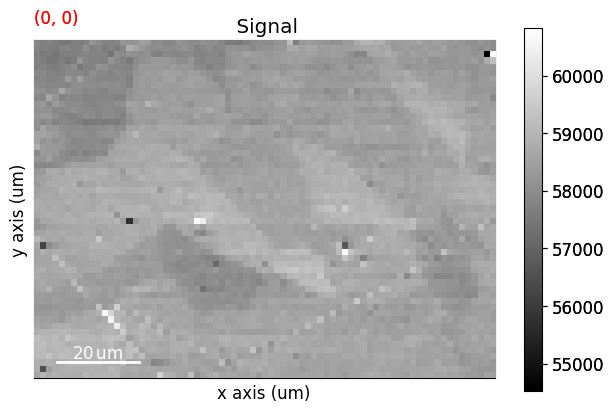
We can set and plot the detector grid on one of the EBSD patterns, also coloring one or more of the grid tiles red, green and blue, as is done in [Nolze et al., 2017], by calling VirtualBSEImager.plot_grid()

vbse_imager.grid_shape

(5, 5)

vbse_imager.grid_shape = (10, 10)
red = [(7, 1), (8, 1), (8, 2), (9, 1), (9, 2)]
green = [(8, 4), (8, 5), (9, 4), (9, 5)]
blue = [(7, 8), (8, 7), (8, 8), (9, 7), (9, 8)]
p = vbse_imager.plot_grid(
    rgb_channels=[red, green, blue],
    visible_indices=True,  # Default
    pattern_idx=(10, 20),  # Default is (0, 0)
)
p

<EBSD, title: patterns Scan 1, dimensions: (|60, 60)>

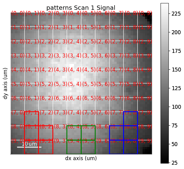
As shown above, whether to show the grid tile indices or not is controlled with the visible_indices argument, and which signal pattern to superimpose the grid upon is controlled with the pattern_idx parameter.

To obtain an RGB image from the detector grid tiles shown above, we use get_rgb_image() (see the docstring for all available parameters)

vbse_rgb_img = vbse_imager.get_rgb_image(r=red, g=green, b=blue)
vbse_rgb_img

<VirtualBSEImage, title: , dimensions: (|75, 55)>

vbse_rgb_img.plot(title="", axes_off=True)

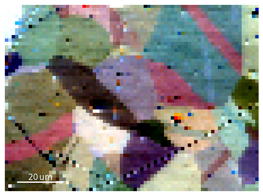
An RGB image formed from coloring three grey scale virtual BSE images red, green and blue.

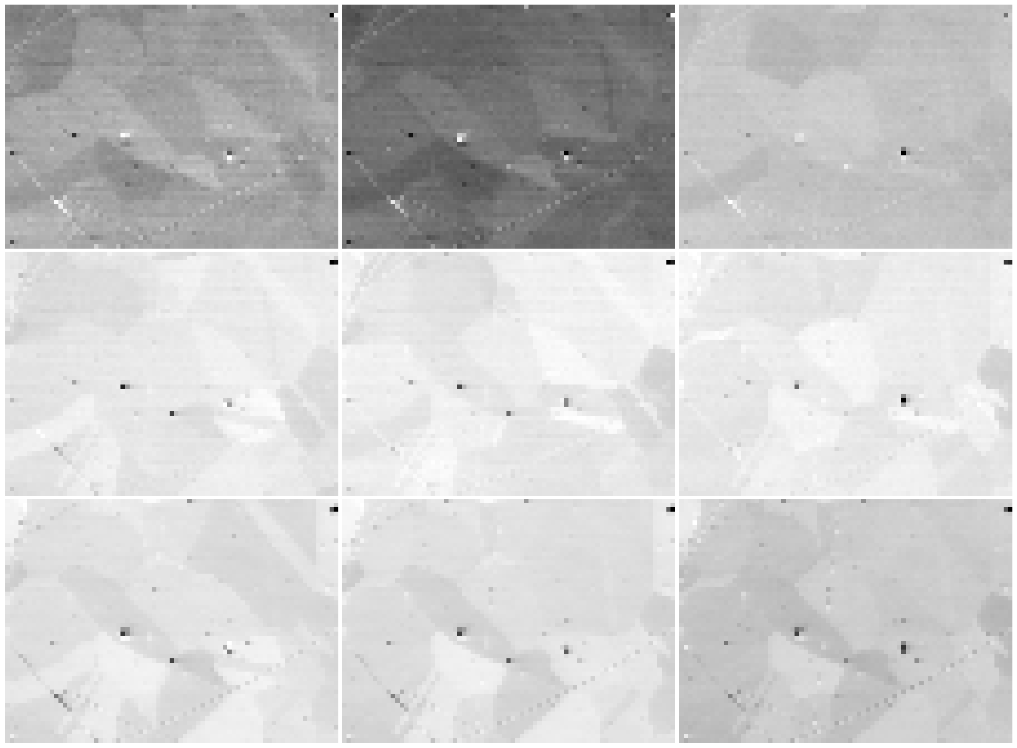
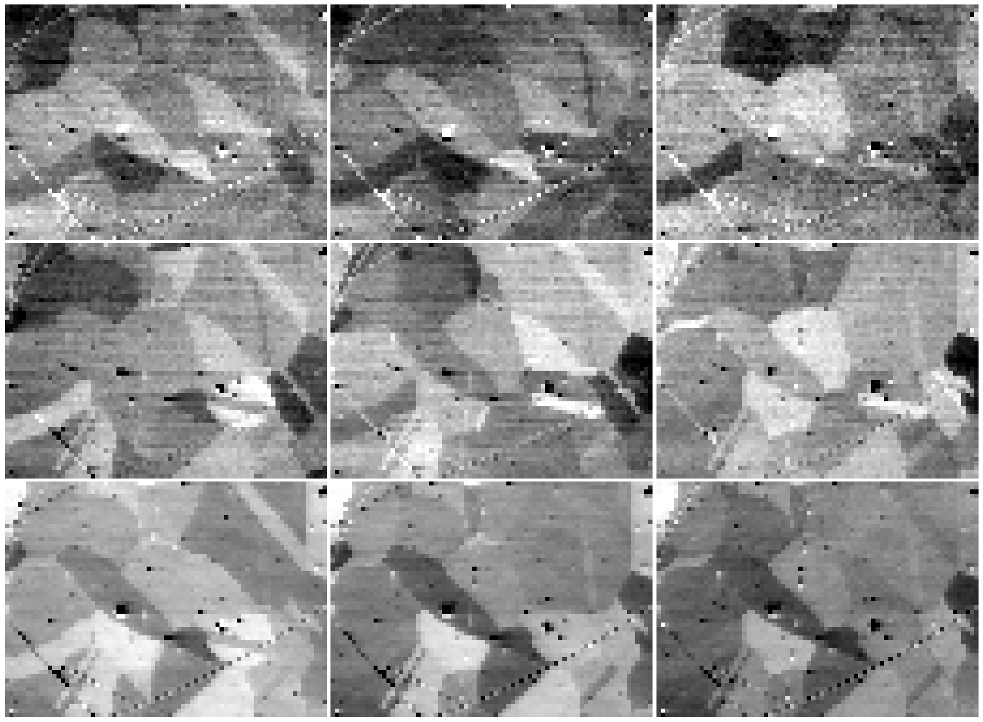
To obtain one grey scale virtual BSE image from each grid tile, we use get_images_from_grid()

vbse_imager.grid_shape = (3, 3)
vbse_imgs = vbse_imager.get_images_from_grid()
vbse_imgs

<VirtualBSEImage, title: , dimensions: (3, 3|75, 55)>

vbse_imgs.plot()

fig, ax = plt.subplots(nrows=3, ncols=3, figsize=(20, 20))
for idx in np.ndindex(vbse_imgs.axes_manager.navigation_shape[::-1]):
    # HyperSpy uses (col, row) instead of NumPy's (row, col)
    hs_idx = idx[::-1]
    ax[idx].imshow(vbse_imgs.inav[hs_idx].data, cmap="gray")
    ax[idx].axis("off")
fig.tight_layout(w_pad=0.5, h_pad=-24)

It might be desirable to normalize, rescale or stretch the intensities in the images, as shown e.g. in Fig. 9 in [Wright et al., 2015]. This can be done with VirtualBSEImage.normalize_intensity() or VirtualBSEImage.rescale_intensity(). Let’s rescale the intensities in each image to the range [0, 1], while also excluding the intensities outside the lower and upper 0.5% percentile, per image

vbse_imgs.data.dtype

dtype('float32')

vbse_imgs2 = vbse_imgs.deepcopy()
vbse_imgs2.rescale_intensity(out_range=(0, 1), percentiles=(0.5, 99.5))

[########################################] | 100% Completed | 115.17 ms

print(vbse_imgs.data.min(), vbse_imgs.data.max())
print(vbse_imgs2.data.min(), vbse_imgs2.data.max())

21321.0 84168.0
-7.962798e-07 1.0000005

fig, ax = plt.subplots(nrows=3, ncols=3, figsize=(20, 20))
for idx in np.ndindex(vbse_imgs2.axes_manager.navigation_shape[::-1]):
    hs_idx = idx[::-1]
    ax[idx].imshow(vbse_imgs2.inav[hs_idx].data, cmap="gray")
    ax[idx].axis("off")
fig.tight_layout(w_pad=0.5, h_pad=-24)

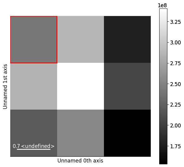
To obtain a rectangular ROI from the grid, we can use VirtualBSEGenerator.roi_from_grid()

roi2 = vbse_imager.roi_from_grid((3, 3))  # (Row, column)
roi2

RectangularROI(left=60, top=60, right=80, bottom=80)