Interactive EBSD detector plotter

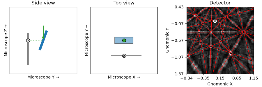
This example shows how to set up an interactive plot showing the side and top view of the microscope as well as the detector plane and the effects of changing detector-sample geometry parameters as well as the crystal orientation.

We use the EBSDDetectorPlotter.

Note

The plotter requires ipywidgets to be installed.

Interactivity is only achieved when run in an active Jupyter session, not directly on this static web page. Run locally with an interactive Matplotlib backend.

Imports.

from diffsims.crystallography import ReciprocalLatticeVector
from IPython.display import display
import matplotlib
import matplotlib.pyplot as plt

import kikuchipy as kp

matplotlib.use("ipympl")
_ = plt.ion()

Load a small (not large) nickel EBSD map.

s = kp.data.nickel_ebsd_large()
print(s)

<EBSD, title: patterns Scan 1, dimensions: (75, 55|60, 60)>

The EBSD dataset has both a crystal map and detector attached.

xmap = s.xmap
print(xmap)

det = s.detector
print(det)

Phase   Orientations  Name  Space group  Point group  Proper point group     Color
    0  4125 (100.0%)    ni        Fm-3m         m-3m                 432  tab:blue
Properties: scores, z
Scan unit: um
EBSDDetector
  shape (Ny, Nx):     (60, 60)
  pc (PCx, PCy, PCz): (0.423, 0.214, 0.502)
  sample_tilt:        70.0°
  tilt:               0.0°
  azimuthal:          0.0°
  twist:              0.0°
  binning:            8
  px_size:            1.0 um

Load the builtin nickel master pattern (of low resolution).

mp = kp.data.nickel_ebsd_master_pattern_small(projection="lambert", energy=20)
print(mp)

<EBSDMasterPattern, title: ni_mc_mp_20kv_uint8_gzip_opts9, dimensions: (|401, 401)>

Set up a reflector list and pick a rotation from the crystal map.

phase = xmap.phases[0]
print(phase)

ref0 = ReciprocalLatticeVector(
    phase=phase, hkl=[[1, 1, 1], [2, 0, 0], [2, 2, 0], [3, 1, 1]]
)
ref0.sanitise_phase()
ref = ref0.symmetrise().unique()

rot = s.xmap.rotations[0]

<name: ni. space group: Fm-3m. point group: m-3m. proper point group: 432. color: tab:blue>

Create a plotter and add the geometrical and dynamical simulations.

pl = kp.draw.EBSDDetectorPlotter(detector=det, rotation=rot, inplace=True)
pl.set_geometrical_simulation(reflectors=ref)
pl.set_master_pattern(mp)
print(pl)

EBSDDetectorPlotter(inplace=True)
  shape (Ny, Nx):     (60, 60)
  pc (PCx, PCy, PCz): (0.423, 0.214, 0.502)
  sample_tilt:        70.0°
  tilt:               0.0°
  azimuthal:          0.0°
  twist:              0.0°
  binning:            8
  px_size:            1.0 um
  Geometrical simulation: ReciprocalLatticeVector (50,), ni (m-3m)
  Master pattern: <EBSDMasterPattern, title: ni_mc_mp_20kv_uint8_gzip_opts9, dimensions: (|401, 401)>

Show the plotter and controls (when run locally).

fig, controls = pl.show(figsize=(9, 3))

display(controls)

plt.show()

HBox(children=(VBox(children=(HTML(value='<b>Detector-sample geometry</b>'), FloatSlider(value=70.0, description='Sample tilt [°]', max=90.0, style=SliderStyle(description_width='initial')), FloatSlider(value=0.0, description='Detector tilt [°]', max=90.0, min=-90.0, style=SliderStyle(description_width='initial')), FloatSlider(value=0.0, description='Azimuthal [°]', max=10.0, min=-10.0, step=0.01, style=SliderStyle(description_width='initial')), FloatSlider(value=0.0, description='Twist [°]', max=10.0, min=-10.0, style=SliderStyle(description_width='initial')), FloatSlider(value=0.4232600661596353, description='PCx', max=1.0, step=0.01, style=SliderStyle(description_width='initial')), FloatSlider(value=0.2136332544638906, description='PCy', max=1.5, min=-0.5, step=0.01, style=SliderStyle(description_width='initial')), FloatSlider(value=0.5020740783903906, description='PCz', max=1.0, min=0.2, step=0.01, style=SliderStyle(description_width='initial')))), VBox(children=(HTML(value='<b>Crystal orientation</b>'), FloatSlider(value=356.4331553036092, description='φ1 [°]', max=360.0, style=SliderStyle(description_width='initial')), FloatSlider(value=94.72125642285175, description='Φ [°]', max=180.0, style=SliderStyle(description_width='initial')), FloatSlider(value=141.77577886513592, description='φ2 [°]', max=360.0, style=SliderStyle(description_width='initial')))), VBox(children=(HTML(value='<b>Overlay</b>'), Checkbox(value=True, description='PC', indent=False), Checkbox(value=False, description='Gnomonic circles', indent=False), Checkbox(value=True, description='Geometric', indent=False), Checkbox(value=True, description='Simulation', indent=False)))))
Canvas(toolbar=Toolbar(toolitems=[('Home', 'Reset original view', 'home', 'home'), ('Back', 'Back to previous view', 'arrow-left', 'back'), ('Forward', 'Forward to next view', 'arrow-right', 'forward'), ('Pan', 'Left button pans, Right button zooms\nx/y fixes axis, CTRL fixes aspect', 'arrows', 'pan'), ('Zoom', 'Zoom to rectangle\nx/y fixes axis', 'square-o', 'zoom'), ('Download', 'Download plot', 'floppy-o', 'save_figure')]))