
Live notebook
You can run this notebook in a live session ![]() or view it on Github.
or view it on Github.
PC calibration: “moving-screen” technique#
The projection center (PC) describing the position of the EBSD detector relative to the beam-sample interaction volume can be estimated by the “moving-screen” technique [Hjelen et al., 1991]. In this tutorial, we test this technique to get a rough estimate of the PC.
The technique assumes that the PC vector from the detector to the sample, shown in the top figure in the reference frames tutorial, is normal to the detector screen as well as the incoming electron beam. It will therefore intersect the screen at a position independent of the detector distance (DD). To find this position, we need two EBSD patterns acquired with a stationary beam but a known difference \(\Delta z\) in DD, say 5 mm.
First, the goal is to find the pattern position that does not shift between the two camera positions, (\(PC_x\), \(PC_y\)). This point can be estimated in fractions of screen width and height, respectively, by selecting the same pattern features in both patterns. The two points of each pattern feature can then be used to form a straight line, and two or more such lines should intersect at (\(PC_x\), \(PC_y\)).
Second, the DD (\(PC_z\)) can be estimated from the same points. After finding the distances \(L_{in}\) and \(L_{out}\) between two points (features) in both patterns (in = operating position, out = 5 mm from operating position), the DD can be found from the relation
where DD is given in the same unit as \(\Delta z\). If also the detector pixel size \(\delta\) is known (e.g. 46 mm / 508 px), \(PC_z\) can be given in the fraction of the detector screen height
where \(N_r\) is the number of detector rows and \(b\) is the binning factor.
Let’s first import necessary libraries
[1]:
# Exchange inline for notebook or qt5 (from pyqt) for interactive plotting
%matplotlib inline

import matplotlib.pyplot as plt
import numpy as np

from diffsims.crystallography import ReciprocalLatticeVector
from orix.crystal_map import PhaseList
import kikuchipy as kp
We will find an estimate of the PC from two single crystal silicon patterns. These are included in the kikuchipy.data module
[2]:
s_in = kp.data.si_ebsd_moving_screen(0, allow_download=True)
s_in.remove_static_background("divide")
s_in.remove_dynamic_background("divide")
s_in.normalize_intensity(dtype_out="float32")

s_out5mm = kp.data.si_ebsd_moving_screen(5, allow_download=True)
s_out5mm.remove_static_background("divide")
s_out5mm.remove_dynamic_background("divide")
s_out5mm.normalize_intensity(dtype_out="float32")
Downloading file 'data/silicon_ebsd_moving_screen/si_out5mm.h5' from 'https://raw.githubusercontent.com/pyxem/kikuchipy-data/bcab8f7a4ffdb86a97f14e2327a4813d3156a85e/silicon_ebsd_moving_screen/si_out5mm.h5' to '/home/docs/.cache/kikuchipy/develop'.
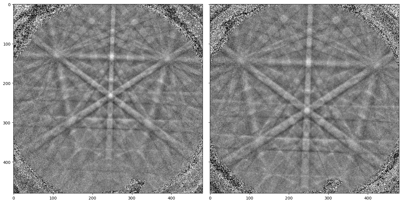
As a first approximation, we can find the detector pixel positions of the same features in both patterns manually with Matplotlib. Cursor pixel coordinates are displayed in the upper right part of the Matplotlib window when plotting with an interactive backend (e.g. qt5 or notebook).
[3]:
fig, axes = plt.subplots(
    ncols=2, sharex=True, sharey=True, figsize=(14, 7), layout="tight"
)
for ax, data in zip(axes, [s_in.data, s_out5mm.data]):
    ax.imshow(data, cmap="gray", vmin=-3, vmax=3)
In this example, we choose the positions of three zone axes. The PC calibration is performed by creating an PCCalibrationMovingScreen instance
[4]:
cal = kp.detectors.PCCalibrationMovingScreen(
    pattern_in=s_in.data,
    pattern_out=s_out5mm.data,
    points_in=[(109, 131), (390, 139), (246, 232)],
    points_out=[(77, 146), (424, 156), (246, 269)],
    delta_z=5,
    px_size=None,  # Default
    convention="tsl",  # Default
)
cal
[4]:
PCCalibrationMovingScreen: (PCx, PCy, PCz) = (0.5123, 0.8606, 21.6518)
3 points:
[[[109. 131.]
  [390. 139.]
  [246. 232.]]

 [[ 77. 146.]
  [424. 156.]
  [246. 269.]]]
We see that (\(PC_x\), \(PC_y\)) = (0.5123, 0.8606), while DD = 21.7 mm. To get \(PC_z\) in fractions of detector height, we have to provide the detector pixel size \(\delta\) upon initialization, or set it directly and recalculate the PC
[5]:
cal.px_size = 90e-3  # mm/px
cal
[5]:
PCCalibrationMovingScreen: (PCx, PCy, PCz) = (0.5123, 0.8606, 0.5012)
3 points:
[[[109. 131.]
  [390. 139.]
  [246. 232.]]

 [[ 77. 146.]
  [424. 156.]
  [246. 269.]]]
We can visualize the estimation by using the convenience method PCCalibrationMovingScreen.plot()
[6]:
cal.plot(pattern_kwargs={"vmin": -3, "vmax": 3, "cmap": "gray"})
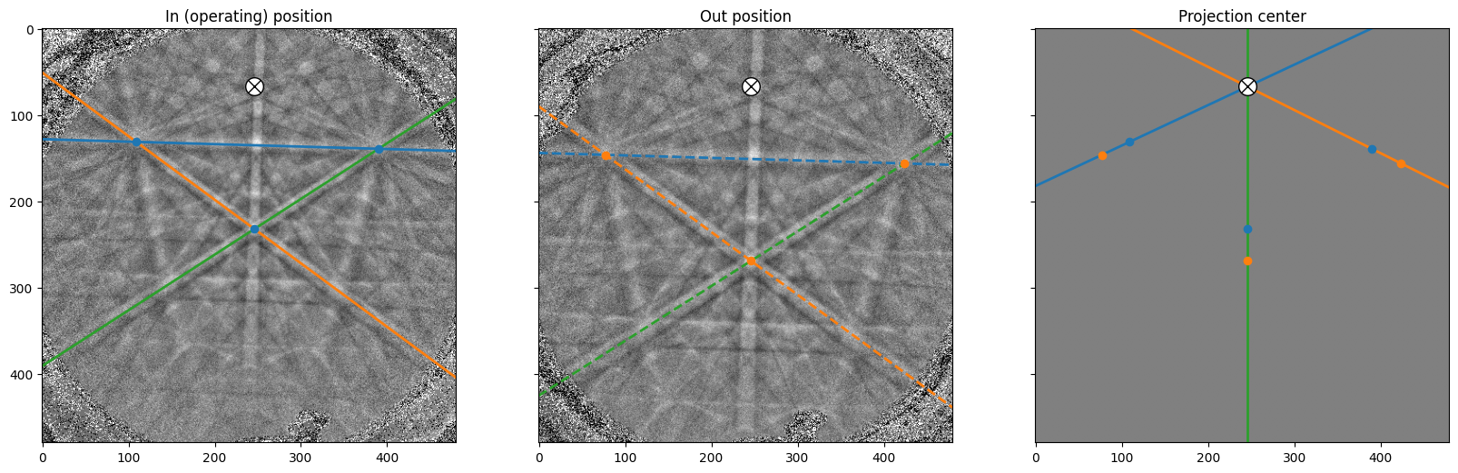
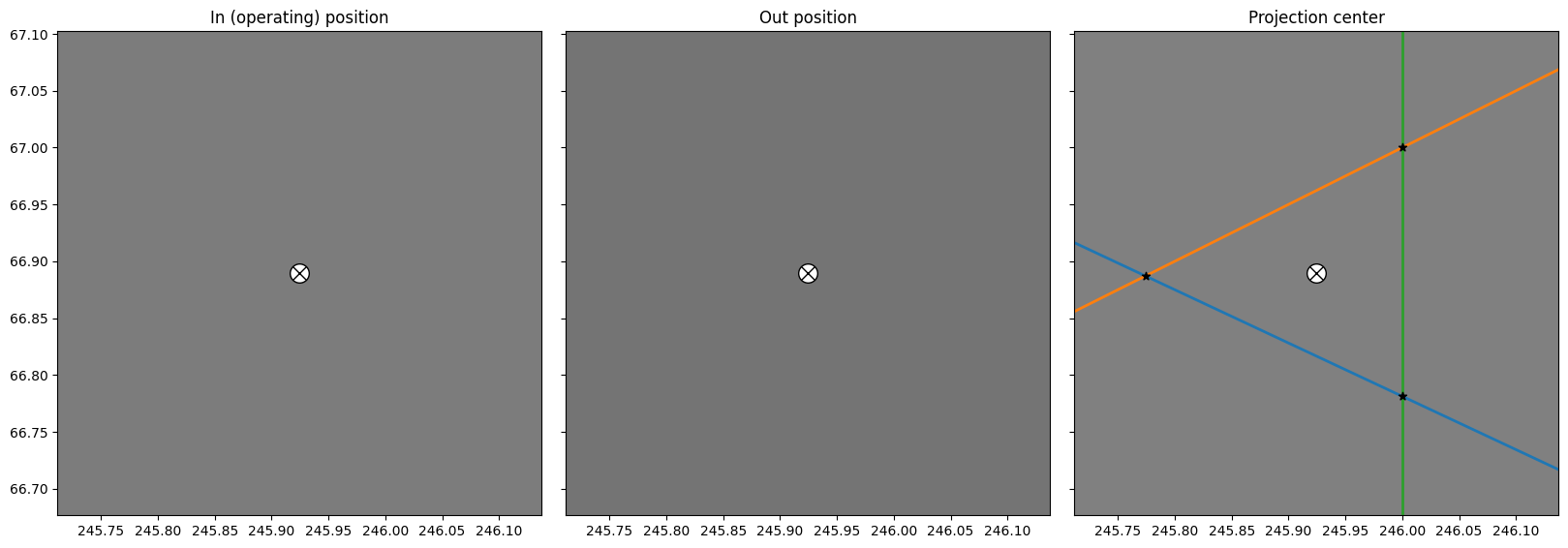
As expected, the three lines in the right figure meet at approimately the same point. We can replot the three images and zoom in on the PC to see how close they are to each other
[7]:
# PCy defined from top to bottom, otherwise "tsl", defined from bottom to top
cal.convention = "bruker"
pcx, pcy, _ = cal.pc

# Use two standard deviations of all $PC_x$ estimates as the axis limits
# (scaled with pattern shape)
two_std = 2 * np.std(cal.pcx_all, axis=0)

fig = cal.plot(return_figure=True)
ax2 = fig.axes[2]
ax2.set_xlim([cal.ncols * (pcx - two_std), cal.ncols * (pcx + two_std)])
ax2.set_ylim([cal.nrows * (pcy - two_std), cal.nrows * (pcy + two_std)])
fig.subplots_adjust(wspace=0.05)
We can use this PC estimate as an initial guess when refining the PC using Hough indexing available from PyEBSDIndex. See the Hough indexing tutorial for details.
Note
PyEBSDIndex is an optional dependency of kikuchipy, and can be installed with both pip and conda (from conda-forge). To install PyEBSDIndex, see their installation instructions.
Create a detector with the correct shape and sample tilt, adding the PC estimate
[8]:
det = kp.detectors.EBSDDetector(cal.shape, sample_tilt=70, pc=cal.pc)
det
[8]:
EBSDDetector
  shape (Ny, Nx):     (480, 480)
  pc (PCx, PCy, PCz): (0.512, 0.139, 0.501)
  sample_tilt:        70.0°
  tilt:               0.0°
  azimuthal:          0.0°
  twist:              0.0°
  binning:            1
  px_size:            1.0 um
Create an EBSDIndexer for use with PyEBSDIndex
[9]:
phase_list = PhaseList(names="si", space_groups=227)
print(phase_list)

indexer = det.get_indexer(phase_list)
Id  Name  Space group  Point group  Proper point group     Color
 0    si        Fd-3m         m-3m                 432  tab:blue
Optimize the PC via Hough indexing and plot the difference between the estimated and optimized PCs
[10]:
n_particles: 30 c1: 3.5 c2: 3.5 w: 0.8
Progress [**********] 50/50  global best:0.207  best loc:[0.5123 0.1465 0.4825]
Optimization finished | best cost: 0.20650988817214966, best pos: [0.51229328 0.14649696 0.48249908]

[[4.99060650e-05 7.14394081e-03 1.86998064e-02]]
Index the pattern via Hough indexing
[11]:
indexer.PC = det_ref.pc

xmap = s_in.hough_indexing(phase_list, indexer=indexer, verbose=2)
Hough indexing with PyEBSDIndex information:
  PyOpenCL: False
  Projection center (Bruker): (0.5123, 0.1465, 0.4825)
  Indexing 1 pattern(s) in 1 chunk(s)
Radon Time: 0.00813424800071516
Convolution Time: 0.0008024779999686871
Peak ID Time: 0.0006929949995537754
Band Label Time: 0.00015588299902447034
Total Band Find Time: 0.00980747399989923
Band Vote Time:  0.001075014000889496
  Indexing speed: 35.31599 patterns/s
Phase  Orientations  Name  Space group  Point group  Proper point group     Color
    0    1 (100.0%)    si        Fd-3m         m-3m                 432  tab:blue
Properties: fit, cm, pq, nmatch
Scan unit: px
[0.20650989]
Create a simulator with the five \(\{hkl\}\) families (reflectors) \(\{111\}\), \(\{200\}\), \(\{220\}\), \(\{222\}\), and \(\{311\}\)
[13]:
ref = ReciprocalLatticeVector(
    phase=xmap.phases[0],
    hkl=[[1, 1, 1], [2, 0, 0], [2, 2, 0], [2, 2, 2], [3, 1, 1]],
)
ref = ref.symmetrise()

simulator = kp.simulations.KikuchiPatternSimulator(ref)

sim = simulator.on_detector(det_ref, xmap.rotations)
Finding bands that are in some pattern:
[########################################] | 100% Completed | 102.06 ms
Finding zone axes that are in some pattern:
[########################################] | 100% Completed | 102.81 ms
Calculating detector coordinates for bands and zone axes:
[########################################] | 100% Completed | 101.93 ms
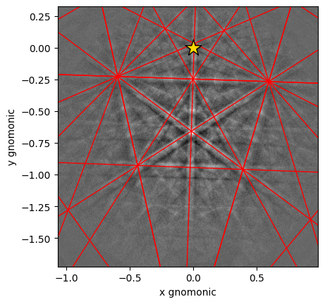
Plot a geometrical simulation on top of the pattern using Kikuchi band centers
[14]:
sim.plot(
    coordinates="gnomonic",
    pattern=s_in.data,
    zone_axes_labels=False,
    zone_axes=False,
    pattern_kwargs={"vmin": -3, "vmax": 3},
)