Live notebook

You can run this notebook in a live session or view it on Github.

Hough indexing

In this tutorial, we will perform Hough/Radon indexing (HI) with PyEBSDIndex. We’ll use a tiny dataset of recrystallized, polycrystalline nickel available with kikuchipy.

Note

PyEBSDIndex is an optional dependency of kikuchipy. It can be installed with both pip and conda (from conda-forge). See their installation instructions for how to install PyEBSDIndex.

Let’s import necessary libraries

# Exchange inline for notebook or qt5 (from pyqt) for interactive plotting
%matplotlib inline

import matplotlib.pyplot as plt
import numpy as np

from diffpy.structure import Atom, Lattice, Structure
from diffsims.crystallography import ReciprocalLatticeVector
import kikuchipy as kp
from orix import io, plot
from orix.crystal_map import Phase, PhaseList
from orix.vector import Vector3d


plt.rcParams.update({"font.size": 15, "lines.markersize": 15})

Load the dataset of (75, 55) nickel EBSD patterns of (60, 60) pixels with a step size of 1.5 μm

s = kp.data.nickel_ebsd_large(allow_download=True)
s

<EBSD, title: patterns Scan 1, dimensions: (75, 55|60, 60)>

Pre-indexing maps

We start by inspecting two indexing-independent maps showing microstructural features: a virtual backscatter electron (VBSE) image and an image quality (IQ) map. The VBSE image gives a qualitative orientation contrast and is created using the BSE yield on the detector. We should use the BSE yield of the raw unprocessed patterns. The IQ map correlates a higher image quality with sharpness of Kikuchi bands. We should thus use processed patterns here.

vbse_imager = kp.imaging.VirtualBSEImager(s)
print(vbse_imager.grid_shape)

(5, 5)

Get the VBSE image by coloring the three grid tiles in the center of the detector red, green, and blue

maps_vbse_rgb = vbse_imager.get_rgb_image(r=(2, 1), g=(2, 2), b=(2, 3))
maps_vbse_rgb

<VirtualBSEImage, title: , dimensions: (|75, 55)>

Plot the VBSE image

maps_vbse_rgb.plot()

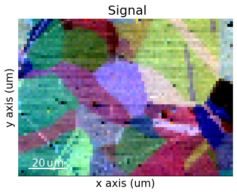
The orientation contrast shows that the region of interest covers 20-30 grains. Several of the grains seem to contain annealing twins.

Enhance the Kikuchi bands by removing the static and dynamic background (see the pattern processing tutorial for details)

s.remove_static_background()
s.remove_dynamic_background()

[########################################] | 100% Completed | 101.53 ms
[########################################] | 100% Completed | 709.09 ms

Get the IQ map

maps_iq = s.get_image_quality()

[########################################] | 100% Completed | 404.74 ms

Plot the IQ map (using the CrystalMap.plot() method of the EBSD.xmap attribute)

s.xmap.plot(
    maps_iq.ravel(),  # Array must be 1D
    cmap="gray",
    colorbar=True,
    colorbar_label="Image quality, $Q$",
    remove_padding=True,
)

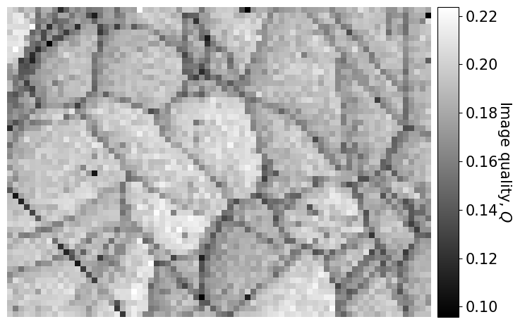
We recognize the boundaries of grains and (presumably) the annealing twins seen in the VBSE image. There are some dark lines, e.g. to the lower and upper left, which look like scratches on the sample surface.

Calibrate detector-sample geometry

Indexing requires knowledge of the position of the sample with respect to the detector. The detector-sample geometry is described by the projection or pattern center (PC) and the tilts of the detector and the sample (see the reference frames tutorial for all conventions). We assume the tilts are known and are thus required input. We will estimate the PC. We do so by optimizing an initial guess of the PC (obtained from similar experiments on the same microscope) using a few selected patterns.

All detector-sample geometry parameters are conveniently stored in an EBSDDetector

sig_shape = s.axes_manager.signal_shape[::-1]  # Make (rows, columns)
det = kp.detectors.EBSDDetector(sig_shape, sample_tilt=70)
det

EBSDDetector (60, 60), px_size 1 um, binning 1, tilt 0, azimuthal 0, pc (0.5, 0.5, 0.5)

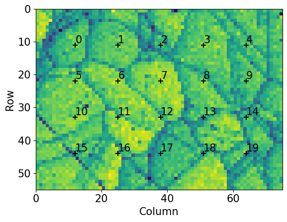
Extract selected patterns from the full dataset. The patterns should be spread out evenly in a map grid to prevent the estimation being biased by diffraction from particular grains or areas of the sample

grid_shape = (5, 4)
s_grid, idx = s.extract_grid(grid_shape, return_indices=True)
s_grid

<EBSD, title: patterns Scan 1, dimensions: (5, 4|60, 60)>

Plot the grid from where the patterns are extracted on the IQ map

nav_shape = s.axes_manager.navigation_shape[::-1]

kp.draw.plot_pattern_positions_in_map(
    rc=idx.reshape(2, -1).T,  # Shape (n patterns, 2)
    roi_shape=nav_shape,  # Or maps_iq.shape
    roi_image=maps_iq,
)

We optimize one PC per pattern in this grid using EBSD.hough_indexing_optimize_pc(). The method calls the PyEBSDIndex function pcopt.optimize() internally. Hough indexing with PyEBSDIndex requires the use of an EBSDIndexer. The indexer stores the list of candidate phases, detector information, and indexing parameters such as the resolution of the Hough transform and the number of bands to use for orientation estimation. We could create this indexer from scratch. Another approach is to get it from an EBSDDetector via EBSDDetector.get_indexer(). This method requires a PhaseList.

We can optionally pass in a list of reflectors per phase (either directly the {hkl} or ReciprocalLatticeVector). The strongest reflectors (bands) for a phase are most likely to be detected in the Radon transform for indexing. Our reflector list should ideally contain these bands. We also need to make sure that our reflector list has enough bands for consistent indexing. This is especially important for multi-phase indexing. We can build up a suitable reflector list with ReciprocalLatticeVector; see e.g. the tutorial on kinematical simulations for how to do this for nickel (point group m-3m), the tetragonal sigma phase in steels (4/mmm), and an hexagonal silicon carbide phase (6mm).

phase_list = PhaseList(
    Phase(
        name="ni",
        space_group=225,
        structure=Structure(
            lattice=Lattice(3.5236, 3.5236, 3.5236, 90, 90, 90),
            atoms=[Atom("Ni", [0, 0, 0])],
        ),
    ),
)
phase_list

Id  Name  Space group  Point group  Proper point group     Color
 0    ni        Fm-3m         m-3m                 432  tab:blue

indexer = det.get_indexer(
    phase_list,
    [[1, 1, 1], [2, 0, 0], [2, 2, 0], [3, 1, 1]],
    nBands=10,
    tSigma=2,
    rSigma=2
)

print(indexer.vendor)
print(indexer.sampleTilt)
print(indexer.camElev)
print(indexer.PC)

print(indexer.phaselist[0].latticeparameter)
print(indexer.phaselist[0].polefamilies)

KIKUCHIPY
70
0
[0.5 0.5 0.5]
[ 3.5236  3.5236  3.5236 90.     90.     90.    ]
[[2 0 0]
 [2 2 0]
 [1 1 1]
 [3 1 1]]

We overwrote the defaults of some of the Hough indexing parameters to use values suggested in PyEBSDIndex’ Radon indexing tutorial:

• tSigma: size of the Gaussian kernel in the \(\theta\) direction in the Radon transform \((\rho, \theta)\)

• rSigma: size of the Gaussian kernel in the \(\rho\) direction

We also set the number of bands to search for in the Radon transform to 10. This is because testing has shown that the default number of 9 can be too few bands for some of the patterns in this dataset.

Now, we can optimize the PCs for each pattern in the extracted grid. (We will “overwrite” the existing detector variable.) We use the particle swarm optimization (PSO) algorithm implemented in PyEBSDIndex The search limit range is set to +/- 0.05 (default is 0.2) since we are sufficiently confident that all PCs are within this range; if we were not, we should increase the search limit.

det = s_grid.hough_indexing_optimize_pc(
    pc0=[0.42, 0.22, 0.50],  # Initial guess based on previous experiments
    indexer=indexer,
    batch=True,
    method="PSO",
    search_limit=0.05,
)

# Print mean and standard deviation
print(det.pc_flattened.mean(axis=0))
print(det.pc_flattened.std(0))

PC found: [**********] 20/20  global best:1.15  PC opt:[0.4343 0.2159 0.5101]
[0.42349787 0.21605024 0.50754341]
[0.00992655 0.00790599 0.00677117]

Plot the PCs

det.plot_pc("scatter", s=50, annotate=True)

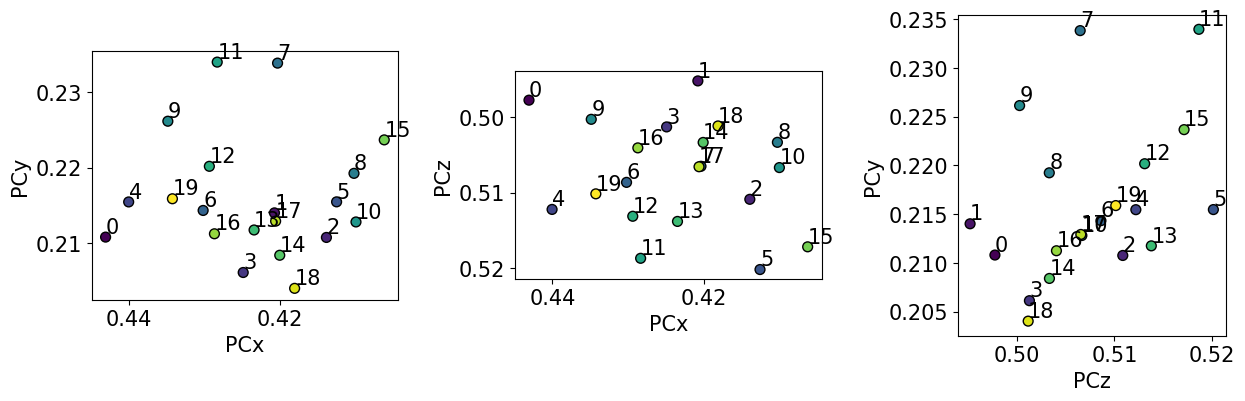
The values do not order nicely in the grid they were extracted from… This is not surprising since they are only (60, 60) pixels wide! Fortunately, the spread is small, and, since the region of interest covers such as small area, we can use the mean PC for indexing.

det.pc = det.pc_average

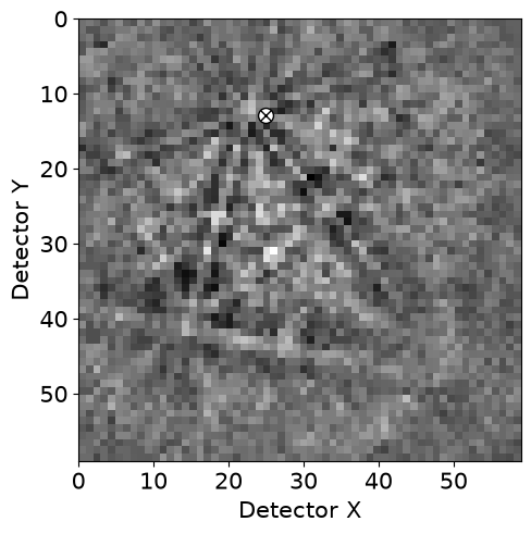
We can check the position of the mean PC on the detector before using it

det.plot(pattern=s_grid.inav[0, 0].data)

Perform indexing

We will index all patterns with this PC calibration. We get a new indexer from the detector with the average PC as determined from the optimization above

indexer = det.get_indexer(
    phase_list,
    [[1, 1, 1], [2, 0, 0], [2, 2, 0], [3, 1, 1]],
    nBands=10,
    tSigma=2,
    rSigma=2
)
indexer.PC

array([0.42349787, 0.21605024, 0.50754341])

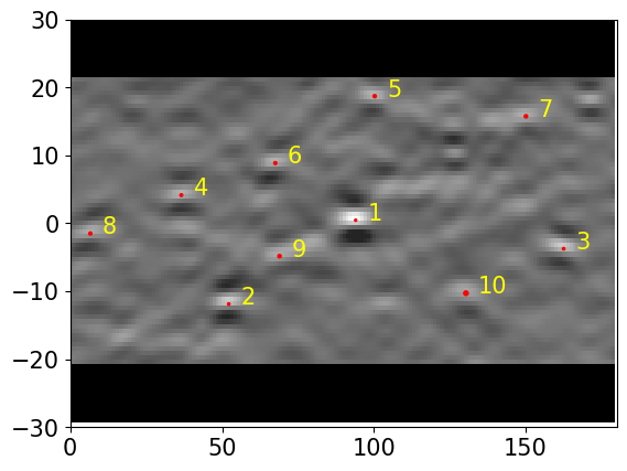
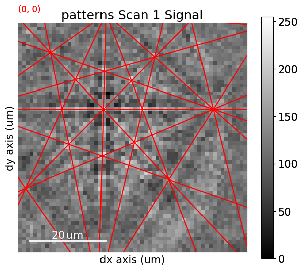
Hough indexing is done with EBSD.hough_indexing(). Since we ask PyEBSDIndex to be “verbose” when reporting on the indexing progress, a figure with the last pattern and its Radon transform is shown. We need to pass the phase list again to EBSD.hough_indexing() (the indexer does not keep all phase information stored in the list [atoms are lost]) for the phases to be described correctly in the returned CrystalMap.

xmap = s.hough_indexing(phase_list=phase_list, indexer=indexer, verbose=2)

Hough indexing with PyEBSDIndex information:
  PyOpenCL: False
  Projection center (Bruker): (0.4235, 0.2161, 0.5075)
  Indexing 4125 pattern(s) in 8 chunk(s)
Radon Time: 6.368019137998999
Convolution Time: 4.452783229999113
Peak ID Time: 3.1347975820008287
Band Label Time: 1.0669431109963625
Total Band Find Time: 15.024665406999702
Band Vote Time:  4.060647591999441
  Indexing speed: 215.81552 patterns/s

xmap

Phase   Orientations  Name  Space group  Point group  Proper point group     Color
    0  4125 (100.0%)    ni        Fm-3m         m-3m                 432  tab:blue
Properties: fit, cm, pq, nmatch
Scan unit: um

We see that all points were indexed as nickel.

Using orix, the indexing results can be exported to an HDF5 file or a text file (.ang) importable by software such as MTEX or other commercial software

#io.save("xmap_ni.h5", xmap)
#io.save(
#    "xmap_ni.ang",
#    xmap,
#    image_quality_prop="pq",
#    confidence_index_prop="cm",
#    extra_prop="nmatch",
#)

Before analyzing the returned orientations, however, we should validate our results.

Validate indexing results

We validate our results by inspecting indexing quality metrics, inverse pole figure (IPF) maps, and comparing geometrical simulations to the experimental patterns.

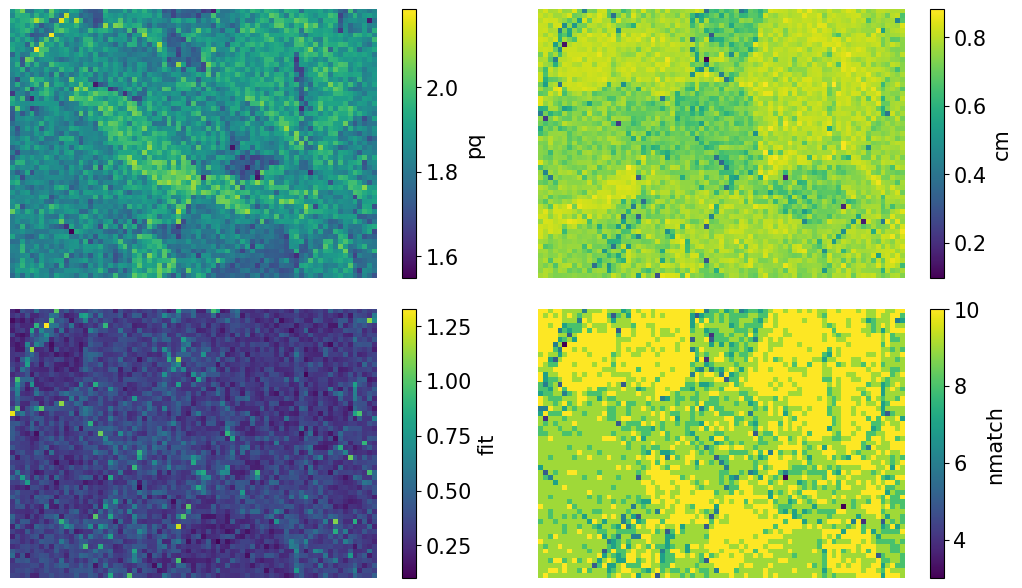
Plot quality metrics

aspect_ratio = xmap.shape[1] / xmap.shape[0]
figsize = (8 * aspect_ratio, 4.5 * aspect_ratio)

fig, axes = plt.subplots(nrows=2, ncols=2, figsize=figsize, layout="tight")
for ax, to_plot in zip(axes.ravel(), ["pq", "cm", "fit", "nmatch"]):
    im = ax.imshow(xmap.get_map_data(to_plot))
    fig.colorbar(im, ax=ax, label=to_plot)
    ax.axis("off")

fig, axes = plt.subplots(ncols=2, nrows=2, figsize=(10, 5), layout="tight")
for ax, to_plot in zip(axes.ravel(), ["pq", "cm", "fit", "nmatch"]):
    ax.hist(xmap.prop[to_plot], bins=100)
    ax.set(xlabel=to_plot, ylabel="Frequency");

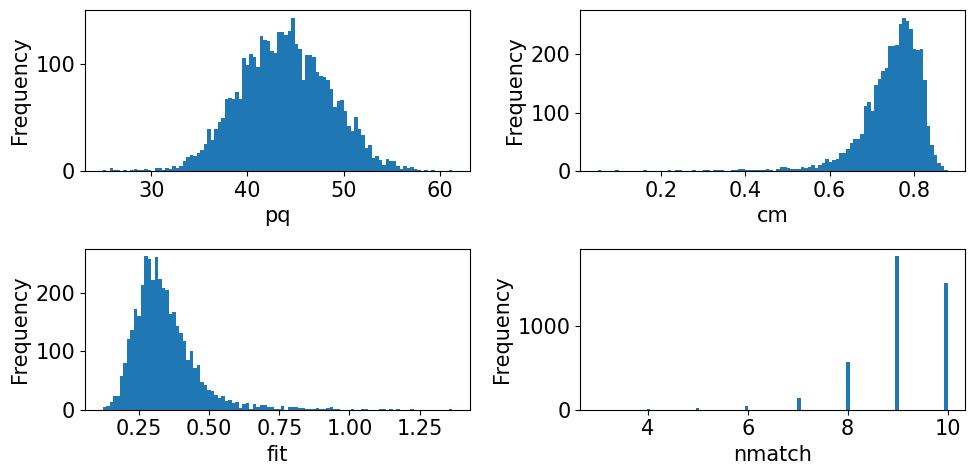
The pattern quality (PQ) and confidence metric (CM) maps show little variation across the sample. The most important map here is that of the pattern fit, also known as the mean angular error/deviation (MAE/MAD): it shows the average angular deviation between the positions of each detected band to the closest “theoretical” band in the indexed solution. The pattern fit is below an OK fit of 1.4\(^{\circ}\) for all patterns. We see that the highest (worst) fit is found in the upper left corner where we recognized some scratches in our IQ map. The final map (nmatch) shows that most detected bands were matched inside most of the grains, with as few as four on some grain boundaries and triple junctions. See PyEBSDIndex’ Radon indexing tutorial for a complete explanation of all the indexing quality metrics.

Create a color key to get IPF colors with

v_ipf = Vector3d.xvector()
sym = xmap.phases[0].point_group

ckey = plot.IPFColorKeyTSL(sym, v_ipf)
ckey

IPFColorKeyTSL, symmetry: m-3m, direction: [1 0 0]

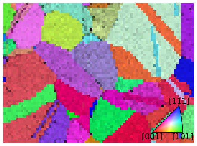
Each point is assigned a color based on which crystal direction \(\left<uvw\right>\) points in a certain sample direction. Let’s plot the IPF-X map with the confidence metric map overlayed

rgb_x = ckey.orientation2color(xmap.rotations)
fig = xmap.plot(rgb_x, overlay="cm", remove_padding=True, return_figure=True)

# Place color key in bottom right corner, coordinates are [left, bottom, width, height]
ax_ckey = fig.add_axes(
    [0.76, 0.08, 0.2, 0.2], projection="ipf", symmetry=sym
)
ax_ckey.plot_ipf_color_key(show_title=False)
ax_ckey.patch.set_facecolor("None")

Let’s also plot the three IPF maps for sample X, Y, and Z side by side

directions = Vector3d(((1, 0, 0), (0, 1, 0), (0, 0, 1)))
n = directions.size

figsize = (4 * n * aspect_ratio, n * aspect_ratio)
fig, ax = plt.subplots(ncols=n, figsize=figsize)
for i, title in zip(range(n), ["X", "Y", "Z"]):
    ckey.direction = directions[i]
    rgb = ckey.orientation2color(xmap.rotations)
    ax[i].imshow(rgb.reshape(xmap.shape + (3,)))
    ax[i].set_title(f"IPF-{title}")
    ax[i].axis("off")
fig.subplots_adjust(wspace=0.02)

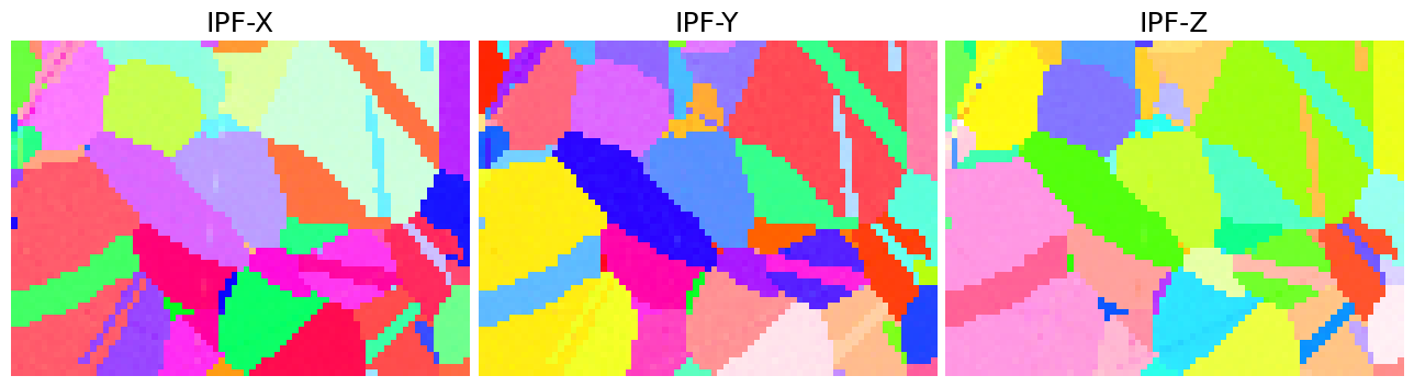
The IPF maps show grains and twins as we expected from the VBSE image and IQ map obtained before indexing.

Plot geometrical simulations on top of the experimental patterns (see the geometrical simulations tutorial for details)

ref = ReciprocalLatticeVector(
    phase=xmap.phases[0], hkl=[[1, 1, 1], [2, 0, 0], [2, 2, 0], [3, 1, 1]]
)
ref = ref.symmetrise()
simulator = kp.simulations.KikuchiPatternSimulator(ref)
sim = simulator.on_detector(det, xmap.rotations.reshape(*xmap.shape))

Finding bands that are in some pattern:
[########################################] | 100% Completed | 101.38 ms
Finding zone axes that are in some pattern:
[########################################] | 100% Completed | 101.97 ms
Calculating detector coordinates for bands and zone axes:
[########################################] | 100% Completed | 101.42 ms

Add markers to EBSD signal

# To remove existing markers
# del s.metadata.Markers

markers = sim.as_markers()
s.add_marker(markers, plot_marker=False, permanent=True)

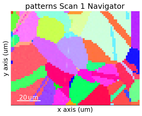
Navigate patterns with simulations in the IPF-X map (see the visualization tutorial for details)

maps_nav_rgb = kp.draw.get_rgb_navigator(rgb_x.reshape(xmap.shape + (3,)))

s.plot(maps_nav_rgb)

What’s next?

If we require a high angular resolution, we might achieve this via refining returned orientations using dynamical simulations. See the refinement section of the pattern matching tutorial for how to do this.

If our validation shows unexpectedly bad results, there are a few key parameters we should look into:

• Phase information: lattice parameters or space group symmetry might be incorrect.

• Detector-sample geometry: sample and detector tilts, but most importantly, the projection center!

• Hough indexing parameters:

  • Reflector list: perhaps the default list or the list passed in by us contain too few reflectors, or they are not the brightest bands for a particular phase?

  • The Gaussian kernel widths for parameters \((\rho, \theta)\) in the Radon transform can affect which bands are detected (wider or narrower). A parameter search might be benefitial.

If we want to speed up Hough indexing, we could try to use PyEBSDIndex’ multi-threading functionality ([see the Radon indexing demo for details).