

Live notebook
You can run this notebook in a live session ![]() or view it on Github.
or view it on Github.
ESTEEM3 workshop#
Note
This tutorial was given at the ESTEEM3 2022 workshop entitled Electron diffraction for solving engineering problems, held at NTNU in Trondheim, Norway in June 2022.
The tutorial has been updated to work with the current release of kikuchipy and to fit our documentation format. The dataset is available from Zenodo at [Ånes et al., 2019], and is scan number 7 (17 dB) out of the series of 10 (22 dB) scans taken with increasing gain (0-22 dB).
In this tutorial we will inspect a small (100 MB) EBSD data of polycrystalline recrystallized nickel by (Hough and dictionary) indexing and inspect the results using geometrical EBSD simulations.
Steps:
Data overview (virtual backscatter electron imaging)
Enhance Kikuchi pattern (background correction)
Data overview (“feature maps”)
Hough indexing
Verification of results (geometrical simulations)
Dictionary indexing
Orientation refinement
Summary
Tools:
kikuchipy: https://kikuchipy.org
HyperSpy: https://hyperspy.org
PyEBSDIndex: https://pyebsdindex.readthedocs.io
diffsims: https://diffsims.readthedocs.io
EMsoft (indirectly): EMsoft-org/EMsoft
Import libraries (replace inline with qt5 plotting backend for interactive plots in separate windows)
[1]:
%matplotlib inline

from pathlib import Path

import matplotlib.pyplot as plt
import numpy as np

from diffsims.crystallography import ReciprocalLatticeVector
import hyperspy.api as hs
import kikuchipy as kp
from orix.crystal_map import CrystalMap, Phase, PhaseList
from orix.quaternion import Orientation, symmetry
from orix import plot, sampling
from orix.vector import Vector3d
from pyebsdindex import ebsd_index, pcopt

plt.rcParams.update(
    {"figure.facecolor": "w", "font.size": 15, "figure.dpi": 75}
)

data_path = Path("../../../kikuchipy_test/esteem")
Load data
[2]:
s = kp.data.ni_gain(7, allow_download=True) # External download
[3]:
[3]:
<EBSD, title: Pattern, dimensions: (200, 149|60, 60)>
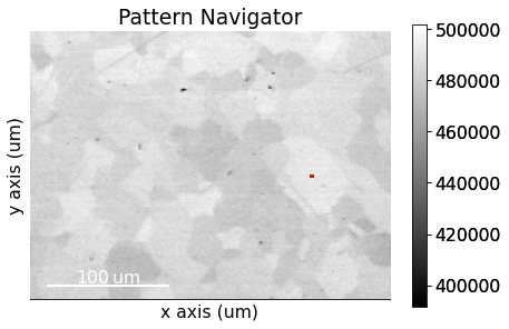
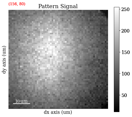
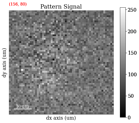
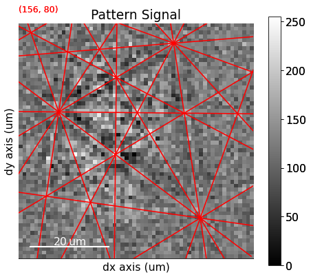
Plot a pattern from a particular grain to show improvement in signal-to-noise ratio
[4]:
s.axes_manager.indices = (156, 80)
Plot data
[5]:
s.plot()

Data overview - virtual imaging#
Mean intensity in each pattern
[6]:
s_mean = s.mean(axis=(2, 3))
s_mean
[6]:
<BaseSignal, title: Pattern, dimensions: (200, 149|)>
Save map
[7]:
# plt.imsave(data_path / "maps_mean.png", s_mean.data, cmap="gray")
Set up VBSE image generator
[8]:
VirtualBSEImager for <EBSD, title: Pattern, dimensions: (200, 149|60, 60)>
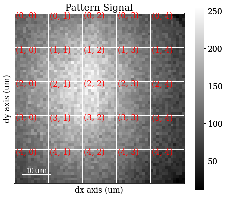
Plot VBSE grid
[9]:
vbse_imager.plot_grid()
[9]:
<EBSD, title: Pattern, dimensions: (|60, 60)>
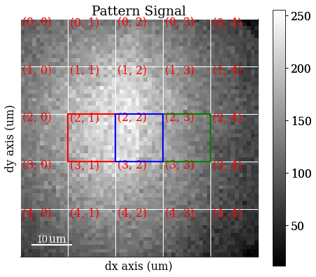
Specify RGB colour channels
[10]:
r = (2, 1)
b = (2, 2)
g = (2, 3)
Plot coloured grid tiles
[11]:
vbse_imager.plot_grid(rgb_channels=[r, g, b])
[11]:
<EBSD, title: Pattern, dimensions: (|60, 60)>
Get VBSE RGB image
[12]:
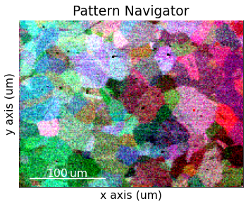
vbse_rgb = vbse_imager.get_rgb_image(r, g, b)
[13]:
s.plot(vbse_rgb)

Save RGB image
[14]:
# vbse_rgb.save(data_path / "maps_vbse_rgb.png")
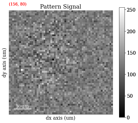
Enhance Kikuchi pattern#
Remove static (constant) background
[15]:
s.remove_static_background()
Inspect statically corrected patterns
[16]:
s.plot(vbse_rgb)
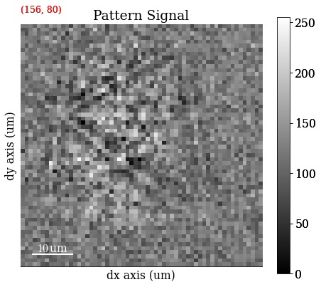
Remove dynamic (per pattern) background
[17]:
s.remove_dynamic_background()
Inspect dynamically corrected patterns
[18]:
s.plot(vbse_rgb)

Average each patterns with the four nearest neighbours
[19]:
s.average_neighbour_patterns()
[########################################] | 100% Completed | 318.13 ms
Inspect average patterns
[20]:
s.plot(vbse_rgb)

Save corrected patterns
[21]:
# s.save(data_path / "patterns_sda.h5")
Data overview - feature maps#
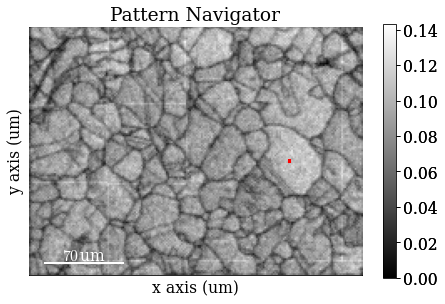
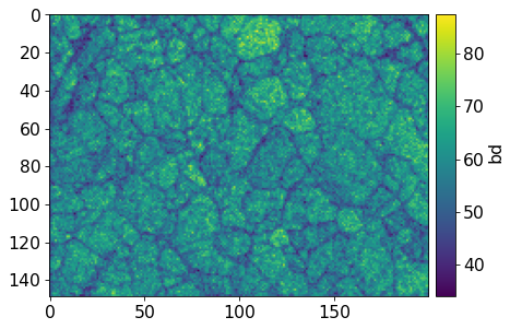
Get image quality \(Q\) map (not image quality IQ from Hough indexing!)
[22]:
maps_iq = s.get_image_quality()
Navigate patterns in \(Q\) map
[23]:
s_iq = hs.signals.Signal2D(maps_iq)
[24]:
s.plot(s_iq)

Save \(Q\) map to file
[25]:
# plt.imsave(data_path / "maps_iq.png", maps_iq, cmap="gray")
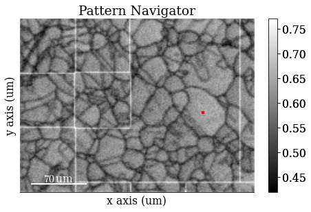
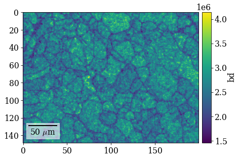
Get average neighbour dot product map (ADP)
[26]:
maps_adp = s.get_average_neighbour_dot_product_map()
[########################################] | 100% Completed | 2.40 ss
Navigate patterns in the ADP map
[27]:
s_adp = hs.signals.Signal2D(maps_adp)
[28]:
s.plot(s_adp)

Save ADP map to file
[29]:
# plt.imsave(data_path / "maps_adp.png", maps_adp, cmap="gray")
Hough indexing of calibration patterns#
Orientation of detector with respect to the sample:
Known:
Sample tilt (about microscope X)
Camera tilt (about microscope X)
Unknown:
Projection/pattern centre (PCx, PCy, PCz): Shortest distance from source point to detector
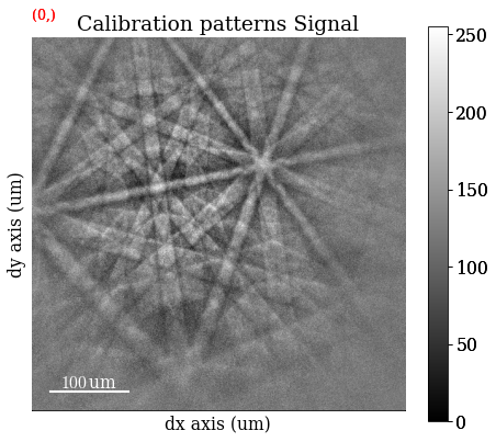
Load calibration patterns to get a mean PC for the data
[30]:
[31]:
[31]:
<EBSD, title: Calibration patterns, dimensions: (9|480, 480)>
[32]:
s_cal.remove_static_background()
s_cal.remove_dynamic_background()
[33]:
s_cal.plot(navigator="none")
Generate an indexer instance used to optimize the PC and to perform Hough indexing
[34]:
sig_shape_cal = s_cal.axes_manager.signal_shape[::-1]
indexer_cal = ebsd_index.EBSDIndexer(
    phaselist=["FCC"],
    vendor="KIKUCHIPY",
    sampleTilt=70,
    camElev=0,
    patDim=sig_shape_cal,
)
Given an initial guess of the PC and optimize for the first calibration pattern, looking for convergence by updating pc0 manually with the printed PC a couple of times (the first run of optimize() takes longer since PyEBSDIndex has to compile some code before running; consecutive runs are much quicker)
[35]:
pc0 = [0.42, 0.21, 0.50]
pc = pcopt.optimize(s_cal.inav[0].data, indexer=indexer_cal, PC0=pc0)
print(pc)
[0.40989986 0.22812557 0.50232882]
Optimize for all calibration patterns
[36]:
pc_all = pcopt.optimize(s_cal.data, indexer_cal, pc, batch=True)
print(pc_all)
[[0.40989986 0.22812557 0.50232882]
 [0.42080225 0.22689171 0.50389273]
 [0.42197546 0.23040527 0.50051151]
 [0.41674551 0.21559051 0.50792767]
 [0.4168258  0.22587122 0.4891827 ]
 [0.42465363 0.21408689 0.50678572]
 [0.40773826 0.2422661  0.49553853]
 [0.4159323  0.21945205 0.5049746 ]
 [0.42625081 0.22599299 0.5010185 ]]
Calculate the mean PC
[0.41786932 0.22540915 0.5013512 ]
[0.00590662 0.00802313 0.00553778]
Index the calibration patterns
[38]:
plt.figure()
hi_res, *_ = indexer_cal.index_pats(s_cal.data, PC=pc_mean, verbose=2)
Radon Time: 0.010707249995903112
Convolution Time: 0.001086707998183556
Peak ID Time: 0.001588416998856701
Band Label Time: 0.0006889579963171855
Total Band Find Time: 0.014083292000577785
Band Vote Time:  0.0029965420108055696
<Figure size 480x360 with 0 Axes>
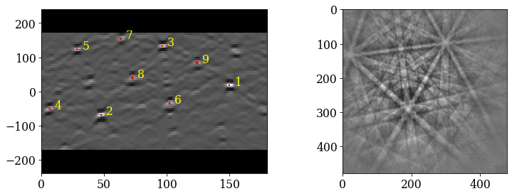
Plot the returned orientations in the inverse pole figure (IPF), showing the crystal direction \([uvw]\) parallel to the out-of-plane direction (Z)
[39]:
O_hi = Orientation(hi_res[-1]["quat"], symmetry.Oh)
O_hi.scatter("ipf")
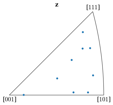
We can determine whether the indexed orientations are correct by projecting geometrical simulations (bands and zone axes) onto the patterns
Geometrical simulations#
Read the typical description of the cubic Nickel phase from a crystallographic information file (CIF)
[40]:
<name: ni. space group: Fm-3m. point group: m-3m. proper point group: 432. color: tab:blue>
[41]:
phase.structure
[41]:
[Ni   0.000000 0.000000 0.000000 1.0000,
 Ni   0.000000 0.500000 0.500000 1.0000,
 Ni   0.500000 0.000000 0.500000 1.0000,
 Ni   0.500000 0.500000 0.000000 1.0000,
 Ni   0.000000 0.500000 0.500000 1.0000,
 Ni   0.500000 0.000000 0.500000 1.0000,
 Ni   0.500000 0.500000 0.000000 1.0000,
 Ni   0.000000 0.000000 0.000000 1.0000,
 Ni   0.500000 0.000000 0.500000 1.0000,
 Ni   0.500000 0.500000 0.000000 1.0000,
 Ni   0.000000 0.500000 0.500000 1.0000,
 Ni   0.000000 0.000000 0.000000 1.0000,
 Ni   0.500000 0.500000 0.000000 1.0000,
 Ni   0.000000 0.500000 0.500000 1.0000,
 Ni   0.500000 0.000000 0.500000 1.0000,
 Ni   0.000000 0.000000 0.000000 1.0000]
[42]:
phase.structure.lattice
[42]:
Lattice(a=3.5058, b=3.5058, c=3.5058, alpha=90, beta=90, gamma=90)
Obtain a set of reflectors \(\mathbf{g}\) with a minimum interplanar spacing \(d\) = 1 Å. Keep the reflectors with a structure factor \(|F| > 0.5 |F|_{\mathrm{max}}\).
[43]:
 h k l      d     |F|_hkl   |F|^2   |F|^2_rel   Mult
 1 1 1    2.024    47.1    2219.7     100.0      8
 2 0 0    1.753    41.4    1715.5      77.3      6
 2 2 0    1.239    29.5     870.2      39.2      12
 3 1 1    1.057    24.7     609.8      27.5      24
Give each distinct set of \(\{hkl\}\) a colour
[44]:
hkl_sets = g.get_hkl_sets()
[45]:
hkl_sets
[45]:
defaultdict(tuple,
            {(np.float64(2.0),
              np.float64(0.0),
              np.float64(0.0)): (array([ 6, 22, 24, 25, 27, 43]),),
             (np.float64(2.0),
              np.float64(2.0),
              np.float64(0.0)): (array([ 4,  5,  7,  8, 21, 23, 26, 28, 41, 42, 44, 45]),),
             (np.float64(1.0),
              np.float64(1.0),
              np.float64(1.0)): (array([12, 13, 16, 17, 32, 33, 36, 37]),),
             (np.float64(3.0),
              np.float64(1.0),
              np.float64(1.0)): (array([ 0,  1,  2,  3,  9, 10, 11, 14, 15, 18, 19, 20, 29, 30, 31, 34, 35,
                     38, 39, 40, 46, 47, 48, 49]),)})
[46]:
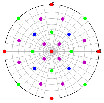
Plot each \((hkl)\) in the stereographic projection
[47]:
g.scatter(c=hkl_rgb, grid=True, s=100, axes_labels=["e1", "e2"])
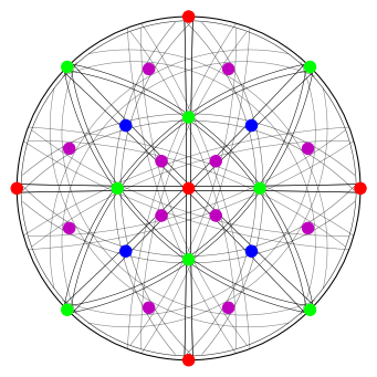
Plot the plane trace of each \((hkl)\) in the stereographic projection
[48]:
g.draw_circle(color=hkl_rgb, axes_labels=["e1", "e2"])

Set up geometrical simulations
[49]:
Calculate Bragg angles and plot bands in the stereographic projection
[50]:
simulator.reflectors.calculate_theta(20e3)
[51]:
fig = simulator.plot(hemisphere="upper", mode="bands", return_figure=True)
fig.axes[0].scatter(g, c=hkl_rgb, s=100)
Specify the detector-sample geometry and perform geometrical simulations on the detector for each orientation found from Hough indexing
[52]:
det_cal = kp.detectors.EBSDDetector(
    shape=sig_shape_cal, pc=pc_mean, sample_tilt=70
)
det_cal
[52]:
EBSDDetector
  shape (Ny, Nx):     (480, 480)
  pc (PCx, PCy, PCz): (0.418, 0.225, 0.501)
  sample_tilt:        70.0°
  tilt:               0.0°
  azimuthal:          0.0°
  twist:              0.0°
  binning:            1
  px_size:            1.0 um
Finding bands that are in some pattern:
[########################################] | 100% Completed | 105.47 ms
Finding zone axes that are in some pattern:
[########################################] | 100% Completed | 106.11 ms
Calculating detector coordinates for bands and zone axes:
[########################################] | 100% Completed | 107.39 ms
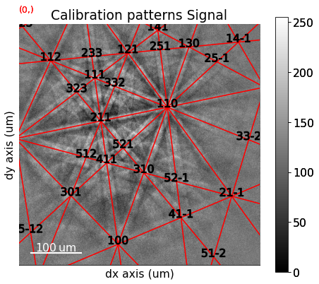
Plot the simulations as markers
[54]:
sim_markers = sim.as_markers(zone_axes_labels=True)
[55]:
s_cal.add_marker(sim_markers, permanent=True, plot_signal=False)
[56]:
s_cal.plot(navigator="none")
[57]:
# To delete previously added permanent markers, do
del s_cal.metadata.Markers
Hough indexing of all patterns#
Create a new indexer and Hough index all patterns
[58]:
sig_shape = s.axes_manager.signal_shape[::-1]
indexer = ebsd_index.EBSDIndexer(
    phaselist=["FCC"],
    vendor="KIKUCHIPY",
    sampleTilt=det_cal.sample_tilt,
    camElev=det_cal.tilt,
    patDim=sig_shape,
)
[59]:
hi_res_all, *_ = indexer.index_pats(
    s.data.reshape((-1,) + sig_shape), PC=det_cal.pc, verbose=2
)
Radon Time: 2.6690933359932387
Convolution Time: 2.172968375016353
Peak ID Time: 7.2510814579582075
Band Label Time: 3.029723333995207
Total Band Find Time: 15.124324500007788
Band Vote Time:  0.4999752500007162

Inspect the first output object (the only one kept)
[60]:
hi_res_all.dtype
[60]:
dtype([('quat', '<f8', (4,)), ('iq', '<f4'), ('pq', '<f4'), ('cm', '<f4'), ('phase', '<i4'), ('fit', '<f4'), ('nmatch', '<i4'), ('matchattempts', '<i4', (4,)), ('totvotes', '<i4')])
Create map coordinate arrays
[61]:
step_size = s.axes_manager["x"].scale
nav_shape = s.axes_manager.navigation_shape[::-1]
i, j = np.indices(nav_shape) * step_size
Contain indexing results in a crystal map for easy plotting and saving
[62]:
xmap_hi = CrystalMap(
    rotations=Orientation(hi_res_all[-1]["quat"]),
    phase_list=PhaseList(phase),
    x=j.ravel(),
    y=i.ravel(),
    prop={
        "pq": hi_res_all[-1]["pq"],
        "cm": hi_res_all[-1]["cm"],
        "fit": hi_res_all[-1]["fit"],
    },
    scan_unit="um",
)
[63]:
[63]:
Phase    Orientations  Name  Space group  Point group  Proper point group     Color
    0  29800 (100.0%)    ni        Fm-3m         m-3m                 432  tab:blue
Properties: pq, cm, fit
Scan unit: um
Plot pattern quality (PC) and confidence metric (CM) maps
[64]:
fig = xmap_hi.plot(
    "pq", colorbar=True, colorbar_label="pq", return_figure=True
)
fig.savefig(data_path / "maps_hi_pq.png")
[65]:
fig = xmap_hi.plot(
    "cm", colorbar=True, colorbar_label="cm", return_figure=True
)
fig.savefig(data_path / "maps_hi_cm.png")
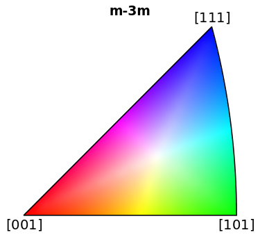
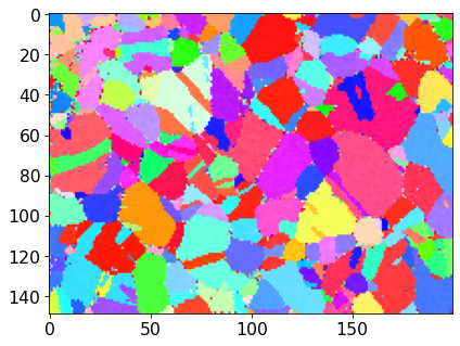
Plot (IPF-X) orientation map
[66]:
ipfkey = plot.IPFColorKeyTSL(
    xmap_hi.phases[0].point_group, direction=Vector3d.xvector()
)
[67]:
fig = ipfkey.plot(return_figure=True)
[68]:
# fig.savefig(data_path / "ipfkey.png")
[69]:
O_hi = xmap_hi.orientations
[70]:
rgb_hi = ipfkey.orientation2color(O_hi)
[71]:
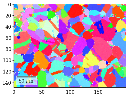
fig = xmap_hi.plot(rgb_hi, return_figure=True)
# fig.savefig(data_path / "maps_hi_ipfz.png")
[72]:
fig = xmap_hi.plot(rgb_hi, overlay=maps_iq.ravel(), return_figure=True)
# fig.savefig(data_path / "maps_hi_ipfz_iq.png")
Save Hough indexing results to file (.ang file readable by MTEX, EDAX TSL OIM Analysis etc., HDF5 file can be read back in into Python)
[73]:
# from orix import io
# io.save(data_path / "xmap_hi.ang", xmap_hi)
[74]:
# io.save(data_path / "xmap_hi.h5", xmap_hi)
Create a new detector with a shape corresponding to the experimental patterns
[75]:
det = det_cal.deepcopy()
det.shape = sig_shape
Get geometrical simulations on this detector for all orientations from the map
[76]:
O_hi_2d = O_hi.reshape(*xmap_hi.shape)
sim_hi = simulator.on_detector(det, O_hi_2d)
Finding bands that are in some pattern:
[########################################] | 100% Completed | 101.29 ms
Finding zone axes that are in some pattern:
[########################################] | 100% Completed | 105.93 ms
Calculating detector coordinates for bands and zone axes:
[########################################] | 100% Completed | 102.64 ms
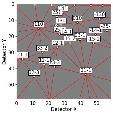
Plot the first simulated pattern
[77]:
sim_hi.plot()
[78]:
rgb_hi_2d = rgb_hi.reshape(xmap_hi.shape + (3,))
s_rgb_hi = kp.draw.get_rgb_navigator(rgb_hi_2d)
Add the geometrical simulations
[79]:
s.add_marker(sim_hi.as_markers(), permanent=True, plot_signal=False)
[80]:
s.plot(s_rgb_hi)
[81]:
# To delete previously added permanent markers, do
del s.metadata.Markers
Dictionary indexing#
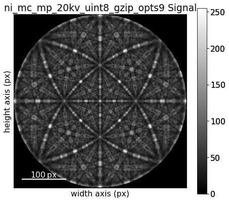
Improve indexing quality by using dynamical simulations. Start by inspecting the dynamically simulated master pattern in the familiar (?) stereographic projection
[82]:
mp_sp = kp.data.nickel_ebsd_master_pattern_small(projection="stereographic")
[83]:
mp_sp.plot()
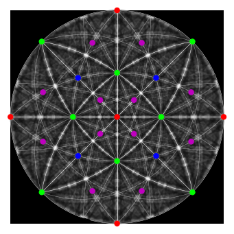
Plot our geometrical simulation on top of the dynamical simulation
[84]:
fig = simulator.plot(
    hemisphere="upper", mode="lines", return_figure=True, color="w"
)
fig.axes[0].scatter(g, c=hkl_rgb, s=50)

fig.axes[0].imshow(mp_sp.data, cmap="gray", extent=(-1, 1, -1, 1));
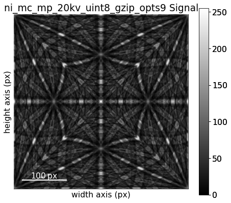
Re-load the master pattern but in the Lambert projection, used to generate the dictionary of dynamically simulated patterns
[85]:
mp = kp.data.nickel_ebsd_master_pattern_small(projection="lambert")
Quickly inspect the Lambert master pattern
[86]:
mp.plot()
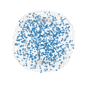
Discretely sample the complete orientation space of point group \(m\bar{3}m\) (Oh) with an average misorientation of about 2.4\(^{\circ}\) between points
[87]:
R_sample = sampling.get_sample_fundamental(
    resolution=2.4, point_group=mp.phase.point_group
)
O_sample = Orientation(R_sample, symmetry=mp.phase.point_group)
[88]:
[88]:
Orientation (58453,) m-3m
[[ 0.8614 -0.3311 -0.3311 -0.1968]
 [ 0.8614 -0.3349 -0.3349 -0.1836]
 [ 0.8614 -0.3384 -0.3384 -0.1703]
 ...
 [ 0.8614  0.3384  0.3384  0.1703]
 [ 0.8614  0.3349  0.3349  0.1836]
 [ 0.8614  0.3311  0.3311  0.1968]]
Plot 1000 sampled orientations in axis-angle space
[89]:
O_sample.get_random_sample(1000).scatter()
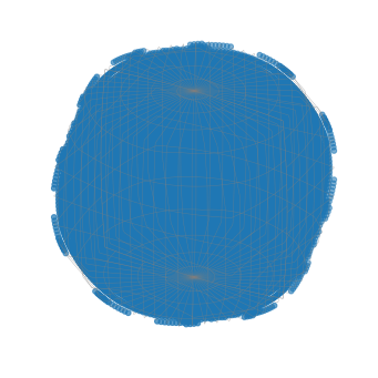
Plot all sampled orientations
[90]:
O_sample.scatter()
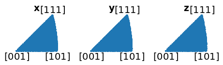
Plot all sampled orientations in the IPFs X, Y, and Z directions
[91]:
directions = Vector3d(((1, 0, 0), (0, 1, 0), (0, 0, 1)))
O_sample.scatter("ipf", direction=directions, c="C0", s=5)
Set up generation of the dictionary of dynamically simulated patterns (with 2 000 patterns per chunk)
[92]:
s_dict = mp.get_patterns(O_sample, det, energy=20, chunk_shape=2000)
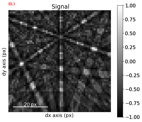
Generate the five first patterns and plot them
[93]:
s_dict.inav[:5].plot(navigator="none")
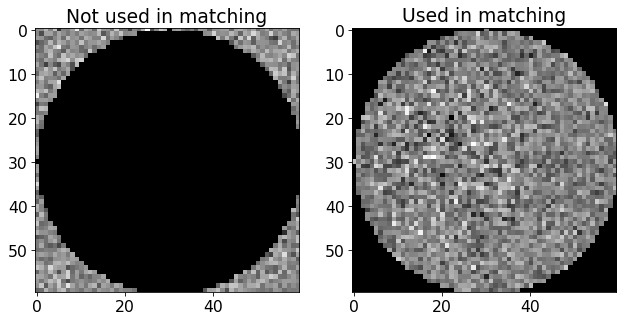
We will use a signal mask so that only pixels with the strongest signal are used during dictionary indexing and refinement
[94]:
signal_mask = ~kp.filters.Window("circular", det.shape).astype(bool)

p = s.inav[0, 0].data
fig, ax = plt.subplots(ncols=2, figsize=(10, 5))
ax[0].imshow(p * signal_mask, cmap="gray")
ax[0].set_title("Not used in matching")
ax[1].imshow(p * ~signal_mask, cmap="gray")
ax[1].set_title("Used in matching");
Perform dictionary indexing by generating 2 000 simulated patterns at a time and compare them to all the experimental patterns
[95]:
xmap_di = s.dictionary_indexing(s_dict, signal_mask=signal_mask)
Dictionary indexing information:
  Phase name: ni
  Matching 29800 experimental pattern(s) to 58453 dictionary pattern(s)
  NormalizedCrossCorrelationMetric: float32, greater is better, rechunk: False, navigation mask: False, signal mask: True
100%|████████████████████████████████████████████████████████████████████████████████████████████████████████████████████████████████████████████████████████████████████████████████| 30/30 [00:40<00:00, 1.34s/it]
Indexing speed: 740.88096 patterns/s, 43306714.69185 comparisons/s
[96]:
xmap_di.scan_unit = "um"
[97]:
[97]:
Phase    Orientations  Name  Space group  Point group  Proper point group     Color
    0  29800 (100.0%)    ni        Fm-3m         m-3m                 432  tab:blue
Properties: scores, simulation_indices
Scan unit: um
[98]:
xmap_di.scores.shape
[98]:
(29800, 20)
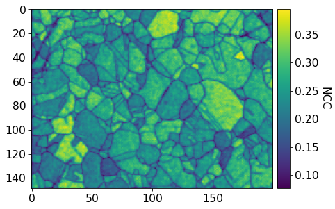
Plot similarity scores (normalized cross-correlation, NCC) between best matching experimental and simulated patterns
[99]:
fig = xmap_di.plot(
    xmap_di.scores[:, 0],
    colorbar=True,
    colorbar_label="NCC",
    return_figure=True,
)
# fig.savefig(data_path / "maps_di_ncc.png")
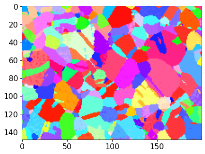
Plot IPF-X orientation map
[100]:
rgb_di = ipfkey.orientation2color(xmap_di.orientations)
[101]:
fig = xmap_di.plot(rgb_di, return_figure=True)
# fig.savefig(data_path / "maps_di_ipfz.png")
Save dictionary indexing results to file
[102]:
# io.save(data_path / "xmap_di.ang", xmap_di)
# io.save(data_path / "xmap_di.h5", xmap_di)
Orientation refinement#
Refine dictionary indexing results by re-generating dynamically simulated patterns iteratively by letting the discretly sampled orientations vary to find the best match
[103]:
Refinement information:
  Method: LN_NELDERMEAD (local) from NLopt
  Trust region (+/-): None
  Relative tolerance: 0.001
Refining 29800 orientation(s):
[########################################] | 100% Completed | 51.73 ss
Refinement speed: 575.63040 patterns/s
[104]:
xmap_ref
[104]:
Phase    Orientations  Name  Space group  Point group  Proper point group     Color
    0  29800 (100.0%)    ni        Fm-3m         m-3m                 432  tab:blue
Properties: scores, num_evals
Scan unit: um
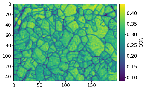
Plot refined NCC scores
[105]:
fig = xmap_ref.plot(
    xmap_ref.scores, colorbar=True, colorbar_label="NCC", return_figure=True
)
# fig.savefig(data_path / "maps_di_ref_ncc.png")
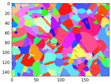
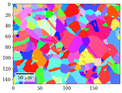
Plot refined IPF-X orientation map
[106]:
rgb_ref = ipfkey.orientation2color(xmap_ref.orientations)
[107]:
fig = xmap_ref.plot(rgb_ref, return_figure=True)
# fig.savefig(data_path / "maps_di_ref_ipfz.png")
[108]:
fig = xmap_ref.plot(rgb_ref, return_figure=True, overlay=xmap_ref.scores)
# fig.savefig(data_path / "maps_di_ref_ipfz_ncc.png")
Save refined results to file
[109]:
# io.save(data_path / "xmap_di_ref.ang", xmap_ref)
# io.save(data_path / "xmap_di_ref.h5", xmap_ref)