Live notebook

You can run this notebook in a live session or view it on Github.

Reference frames

In this tutorial, we will learn of the reference frames most important to EBSD, which conventions are used in kikuchipy, and how these relate to conventions in the other softwares Bruker, EDAX TSL, EMsoft, and Oxford Instruments. We will also test the conversions between these conventions by indexing simulated patterns using Hough indexing (HI) from PyEBSDIndex.

Detector-sample geometry

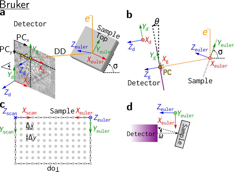
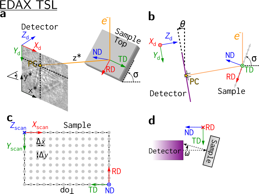
The figure below shows the sample reference frame and the detector reference frame used in kikuchipy, all of which are right handed. In short, the sample reference frame (\(X_s\), \(Y_s\), \(Z_s\)) is the one used by EDAX TSL, (RD, TD, ND), while the pattern center (\(PC_x\), \(PC_y\), \(PC_z\)) is the one used by Bruker Nano, (\(PC_x\), \(PC_y\), \(DD\)).

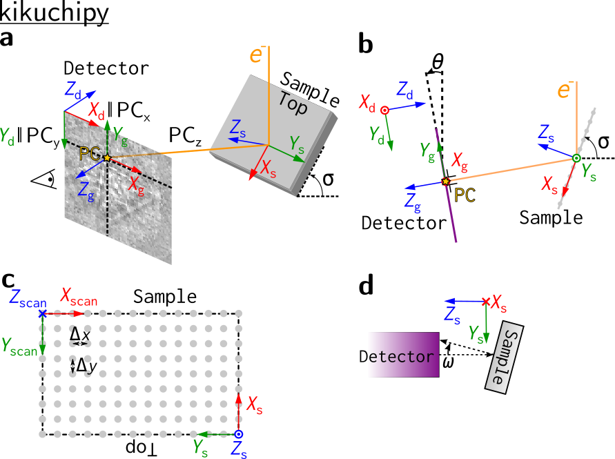
In a, the electron beam interacts with the sample in the source point, and the shortest distance from this point to the detector is called the projection/pattern center (PC). A part of the Kikuchi sphere resulting from the beam-sample interaction is projected onto the flat detector in the gnomonic projection, the EBSD pattern (EBSP). A gnomonic coordinate system \(CS_g\), (\(X_g\), \(Y_g\), \(Z_g\)) with (0, 0, 0) in the PC is defined for the detector plane. We also define a detector coordinate system \(CS_d\), (\(X_d\), \(Y_d\), \(Z_d\)), for the detector plane, with (0, 0, 0) in the upper left corner. The projection center coordinates (\(PC_x\), \(PC_y\), \(PC_z\)) are defined in this detector coordinate system:

• \(PC_x\) is measured from the left border of the detector in fractions of detector width.

• \(PC_y\) is measured from the top border of the detector in fractions of detector height.

• \(PC_z\) is the distance from the detector scintillator to the sample divided by pattern height.

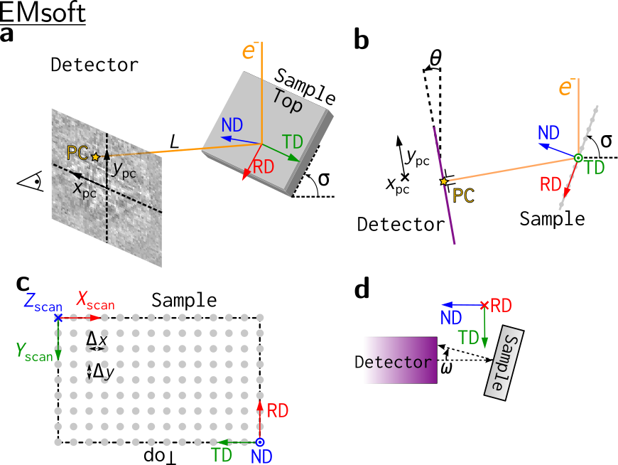
Orientations are defined in the Bunge convention with respect to the sample coordinate system \(CS_s\), (\(X_s\), \(Y_s\), \(Z_s\)). The detector and sample viewed along the microscope \(X\) axis are shown in b, with the three coordinate systems and the PC also shown. The scanned map is shown in c. Note the orientation of \(CS_s\) and the sample “Top”: the map is scanned from the bottom of the sample and upwards. Three tilt angles are defined: the sample tilt \(\sigma\) shown in a and b; the detector tilt \(\theta\) shown in b; the azimuthal angle \(\omega\) which is defined as the sample tilt angle around the \(X_s\) axis, shown in a top view of the detector and sample along the microscope \(Z\) axis in d.

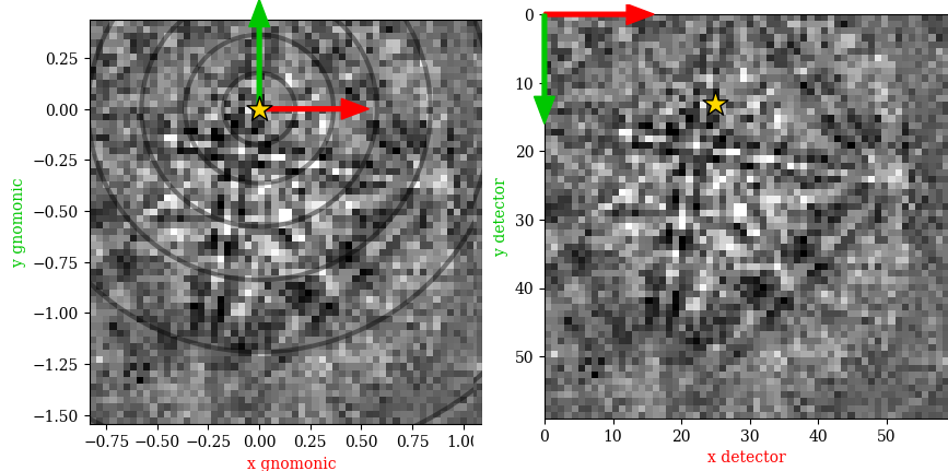
The above figure shows the EBSP in the sample reference frame figure a as viewed from behind the screen towards the sample in (left) the gnomonic coordinate system with its origin (0, 0) in the PC, and in (right) the detector coodinate system with (0, 0) in the upper left pixel. The circles indicate the angular distance from the PC in steps of \(10^{\circ}\).

The EBSD detector

All relevant parameters for the detector-sample geometry are stored in an kikuchipy.detectors.EBSDDetector instance. Let’s first import necessary libraries and a small Nickel EBSD test data set

# Exchange inline for notebook or qt5 (from pyqt) for interactive plotting
%matplotlib inline

import matplotlib.pyplot as plt
import numpy as np

import kikuchipy as kp
from orix.quaternion import Orientation, Rotation
from orix.vector import Vector3d


plt.rcParams["figure.figsize"] = (15, 5)

# Use kp.load("data.h5") to load your own data
s = kp.data.nickel_ebsd_small()
s

2023-06-09 17:11:54,121 - hyperspy.extensions - INFO - Enabling extension kikuchipy

<EBSD, title: patterns Scan 1, dimensions: (3, 3|60, 60)>

Then we can define a detector with the same parameters as the one used to acquire the small Nickel data set

det = kp.detectors.EBSDDetector(
    shape=s.axes_manager.signal_shape[::-1],
    pc=[0.4221, 0.2179, 0.4954],
    px_size=70,  # Microns
    binning=8,
    tilt=0,
    sample_tilt=70,
)
det

EBSDDetector (60, 60), px_size 70 um, binning 8, tilt 0, azimuthal 0, pc (0.422, 0.218, 0.495)

det.pc_tsl()

array([[0.4221, 0.7821, 0.4954]])

Above, the PC was passed in the Bruker convention. Passing the PC in the EDAX TSL, Oxford, or EMsoft convention is also supported. The definitions of the conventions are given in the EBSDDetector API reference, together with the conversion from PC coordinates in the EDAX TSL, Oxford, or EMsoft conventions to PC coordinates in the Bruker convention.

The PC coordinates in the EDAX TSL, Oxford, or EMsoft conventions can be retreived via EBSDDetector.pc_tsl(), EBSDDetector.pc_oxford(), and EBSDDetector.pc_emsoft(), respectively. The latter requires the unbinned detector pixel size in microns and the detector binning to be given upon initialization.

det.pc_emsoft()

array([[   37.392,   135.408, 16645.44 ]])

The detector can be plotted to show whether the average PC is placed as expected using EBSDDetector.plot() (see its docstring for a complete explanation of its parameters)

det.plot(pattern=s.inav[0, 0].data)

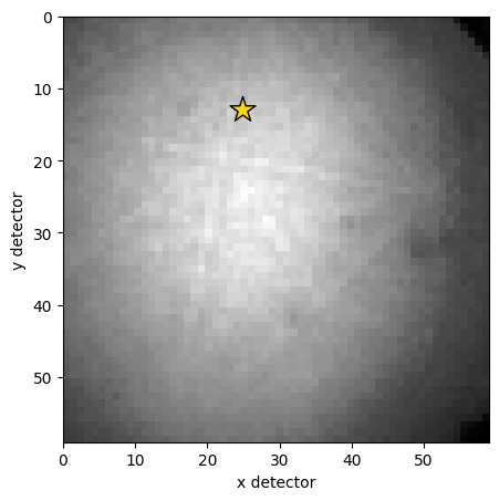
This will produce a figure similar to the right panel in the detector coordinates figure above, without the arrows and colored labels.

Multiple PCs with a 1D or 2D navigation shape can be passed to the pc parameter upon initialization, or can be set directly. This gives the detector a navigation shape (not to be confused with the detector shape) and a navigation dimension (maximum of two)

det.pc = np.ones([3, 4, 3]) * det.pc
det.navigation_shape

(3, 4)

det.navigation_dimension

2

det.navigation_size

12

det.pc = det.pc[0, 0]
det.navigation_shape

(1,)

Note

The offset and scale of HyperSpy’s axes_manager is fixed for a signal, meaning that we cannot let the PC vary with scan position if we want to calibrate the EBSD detector via the axes_manager. The need for a varying PC was the main motivation behind the EBSDDetector class.

The left panel in the detector coordinates figure above shows the detector plotted in the gnomonic projection using EBSDDetector.plot(). The 2D gnomonic coordinates (\(x_g, y_g\)) in \(CS_g\) are defined in \(CS_d\) are

\[x_g = \frac{x_d}{z_d}, \qquad y_g = \frac{y_d}{z_d}.\]

The detector bounds and pixel scale in this projection, per navigation point, are stored with the detector

det.bounds

array([ 0, 59,  0, 59])

det.gnomonic_bounds

array([[-0.85203876,  1.1665321 , -1.57872426,  0.43984659]])

det.x_range

array([[-0.85203876,  1.1665321 ]])

det.r_max  # Largest radial distance to PC

array([[1.96294866]])

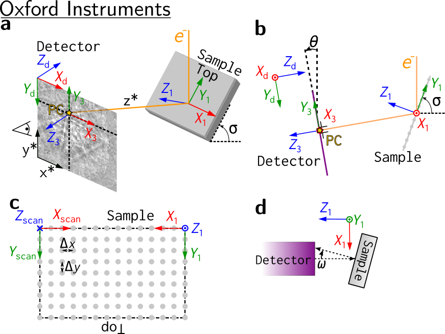
Other software’s reference frames

Other software use other reference frames. To aid in the conversion of a set of observations, typically orientations, between softwares, the reference frames used in other softwares are also shown here, represented to the best of the contributors understanding.

Warning

Reference frames used in other softwares given here are based on instruction manuals from the internet. Use with care, and double check whenever possible.

EMsoft

Bruker

EDAX TSL

Oxford Instruments

Test PC conventions with PyEBSDIndex

We can test the PC conventions using Hough indexing in PyEBSDIndex. We will use ten simulated nickel patterns with a fixed PC and random orientations. We check for consistency by passing the PC in all the conventions described above when indexing, and making sure that the indexed orientations are rotated so that they are defined with respect to the same sample reference frame (the one used in kikuchipy, EDAX TSL and EMsoft).

Note

PyEBSDIndex is an optional dependency of kikuchipy, and can be installed with both pip and conda (from conda-forge). To install PyEBSDIndex, see their installation instructions.

PyEBSDIndex supports indexing face centered and body centered cubic (FCC and BCC) materials.

Load master pattern in the square Lambert projection

mp = kp.data.nickel_ebsd_master_pattern_small(
    projection="lambert", hemisphere="upper"
)

Define a rectangular EBSD detector to project simulated patterns onto

det2 = kp.detectors.EBSDDetector(
    (100, 120), pc=(0.4, 0.2, 0.5), sample_tilt=70
)
det2

EBSDDetector (100, 120), px_size 1 um, binning 1, tilt 0, azimuthal 0, pc (0.4, 0.2, 0.5)

Create ten random orientations

rot = Rotation.random(10)
ori = Orientation(rot, mp.phase.point_group)

Project patterns onto detector

s2 = mp.get_patterns(rot, det2, energy=20, compute=True)

[########################################] | 100% Completed | 102.13 ms

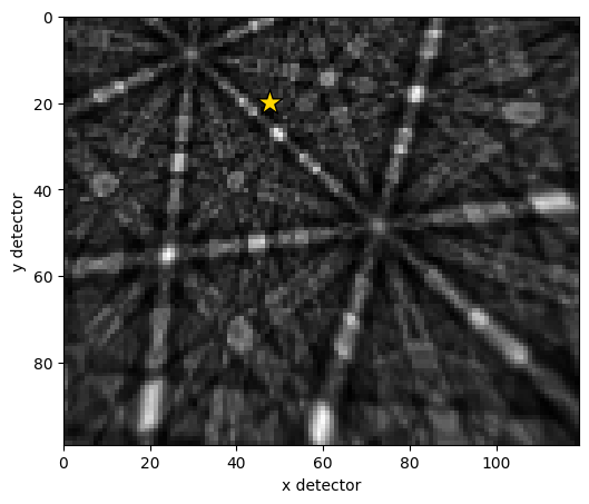
Plot the first simulated pattern and the PC

det2.plot(pattern=s2.inav[0].data)

Load necessary PyEBSDIndex modules for Hough indexing

from pyebsdindex import ebsd_index, pcopt

For the various softwares, define the PCs and the transformations bringing the indexed orientations returned from PyEBSDIndex back to the sample reference frame used in kikuchipy, EDAX TSL and EMsoft

pcs = {
    "KIKUCHIPY": det2.pc,
    "BRUKER": det2.pc,
    "EDAX": det2.pc_tsl(),
    "OXFORD": det2.pc_oxford(),
    "EMSOFT": det2.pc_emsoft(),
}
post_rot = {
    "KIKUCHIPY": Rotation.identity(),
    "BRUKER": Rotation.from_axes_angles((0, 0, 1), -np.pi / 2),
    "EDAX": Rotation.identity(),
    "OXFORD": Rotation.from_axes_angles((0, 0, 1), -np.pi / 2),
    "EMSOFT": Rotation.identity(),
}

# Some wrangling to display a nice table
for softw, pc_i in pcs.items():
    print(
        f"{softw:<9} {pc_i[0, 0]:>6.3f} {pc_i[0, 1]:>6.3f} {pc_i[0, 2]:>6.3f}"
    )

KIKUCHIPY  0.400  0.200  0.500
BRUKER     0.400  0.200  0.500
EDAX       0.400  0.667  0.417
OXFORD     0.400  0.667  0.417
EMSOFT    12.000 30.000 50.000

Then we do the following in a loop:

1. Initialize a PyEBSDIndex indexer, specifying the vendor and vendor specific PC

2. Index the ten patterns

3. Apply vendor specific post rotation to the returned orientations

4. Print misorientation angle between indexed orientations and ground truth orientations

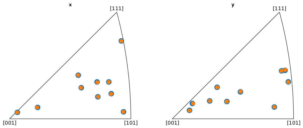
5. Plot the indexed orientations and the ground truth in inverse pole figures (IPFs)

# Keyword arguments common to all vendors
v_sample = Vector3d([(1, 0, 0), (0, 1, 0), (0, 0, 1)])
for vendor, pc in pcs.items():
    print(vendor)

    if vendor == "EMSOFT":
        # PyEBSDIndex requires that the pixel size is passed as the forth PC
        # value in order to correctly scale the L (PCz) parameter to obtain the
        # PC used internally in PyEBSDIndex
        pc = np.append(pc, [1])

    indexer = ebsd_index.EBSDIndexer(
        vendor=vendor,
        PC=pc,
        sampleTilt=det2.sample_tilt,
        camElev=det2.tilt,
        patDim=det2.shape,
    )
    data, *_ = indexer.index_pats(s2.data)
    rot_hi = Rotation(data[-1]["quat"]) * post_rot[vendor]
    ori_hi = Orientation(rot_hi, mp.phase.point_group)

    print("Mori. angle to ground truth:", ori_hi.angle_with(ori, degrees=True))
    fig = ori.scatter(
        "ipf",
        direction=v_sample,
        c="b",
        s=200,
        return_figure=True,
    )
    ori_hi.scatter("ipf", figure=fig, c="orange", s=100)
    plt.pause(0.5)  # Show IPFs before continuing with next vendor

KIKUCHIPY
Mori. angle to ground truth: [0.10794509 0.10128114 0.02586746 0.30046467 0.17063017 0.15398356
 0.18230075 0.21676291 0.12364458 0.21290904]

BRUKER
Mori. angle to ground truth: [0.10794509 0.10128114 0.02586746 0.30046467 0.17063017 0.15398356
 0.18230075 0.21676291 0.12364458 0.21290904]

EDAX
Mori. angle to ground truth: [0.10794509 0.10128114 0.02586746 0.30046467 0.17063017 0.15398356
 0.18230075 0.21676291 0.12364458 0.21290904]

OXFORD
Mori. angle to ground truth: [0.10794509 0.10128114 0.02586746 0.30046467 0.17063017 0.15398356
 0.18230075 0.21676291 0.12364458 0.21290904]

EMSOFT
Mori. angle to ground truth: [0.10794509 0.10128114 0.02586746 0.30046467 0.17063017 0.15398356
 0.18230075 0.21676291 0.12364458 0.21290904]

From the IPFs, we see that all indexed orientations for all vendors are very close to the ground truth orientations, with an average misorientation angle below 0.5\(^{\circ}\). This confirms that the PC conventions for the various vendors shown above are consistent, and that PyEBSDIndex is consistent with kikuchipy.